My aim with this analysis is to get centile curves of WMH and related markers as well as respective z-scores for downstream predictive modelling in a sample from two cohorts.
import pickle
from pcntoolkit.normative import evaluate
import matplotlib.pyplot as plt

import seaborn as sns
sns.set(style='whitegrid')

# random jitter function
def rand_jitter(arr):
    stdev = .005 * (max(arr) - min(arr))
    return arr + np.random.randn(len(arr)) * stdev

for idp_num, c in enumerate(feature_columns):

    if c in tracts_wo_wmh: continue
    print('Running IDP', idp_num, c, ':')
    roi_path = rois_path/c
    os.chdir(roi_path)

    # load the true data points
    X_te = np.loadtxt(os.path.join(roi_path, 'cov_bspline.txt'))
    yhat_te = np.loadtxt(os.path.join(roi_path, 'yhat_estimate.txt'))[:, np.newaxis]
    s2_te = np.loadtxt(os.path.join(roi_path, 'ys2_estimate.txt'))[:,np.newaxis]
    y_te = np.loadtxt(os.path.join(roi_path, f'resp_{c}.txt'))[:,np.newaxis]

    # set up the covariates for the dummy data
    print('Making predictions with dummy covariates (for visualisation)')
    yhat, s2 = ptk.normative.predict(cov_file_dummy,
                       alg = 'blr',
                       respfile = None,
                       model_path = os.path.join(roi_path,'Models'),
                       binary=False,
                       outputsuffix = '_dummy',
                       saveoutput = True,
                       warp="WarpSinArcsinh",
                       warp_reparam=True)

    # load the normative model
    with open(os.path.join(roi_path,'Models', 'NM_0_0_estimate.pkl'), 'rb') as handle:
        nm = pickle.load(handle)

   # get the warp and warp parameters
    W = nm.blr.warp
    warp_param = nm.blr.hyp[1:nm.blr.warp.get_n_params()+1]

    # first, we warp predictions for the true data and compute evaluation metrics
    med_te = W.warp_predictions(np.squeeze(yhat_te), np.squeeze(s2_te), warp_param)[0]
    med_te = med_te[:, np.newaxis]
    print('metrics:', evaluate(y_te, med_te))

    # then, we warp dummy predictions to create the plots
    med, pr_int = W.warp_predictions(np.squeeze(yhat), np.squeeze(s2), warp_param)

    # extract the different variance components to visualise
    beta, junk1, junk2 = nm.blr._parse_hyps(nm.blr.hyp, X_dummy)
    s2n = 1/beta # variation (aleatoric uncertainty)
    s2s = s2-s2n # modelling uncertainty (epistemic uncertainty)

    # plot the data points
    y_te_rescaled_all = np.zeros_like(y_te)
    for sid, site in enumerate(site_ids_te):
        # plot the true test data points
        if all(elem in site_ids_tr for elem in site_ids_te):
            # all data in the test set are present in the training set

            # first, we select the data points belonging to this particular sex and site
            idx = np.where(np.bitwise_and(X_te[:,2] == sex, X_te[:,sid+len(cols_cov)+1] !=0))[0]
            if len(idx) == 0:
                print('No data for site', sid, site, 'skipping...')
                continue

            # then directly adjust the data
            idx_dummy = np.bitwise_and(X_dummy[:,1] > X_te[idx,1].min(), X_dummy[:,1] < X_te[idx,1].max())
            y_te_rescaled = y_te[idx] - np.median(y_te[idx]) + np.median(med[idx_dummy])
        else:
            # we need to adjust the data based on the adaptation dataset

            # first, select the data point belonging to this particular site
            idx = np.where(np.bitwise_and(X_te[:,2] == sex, (df_te['site'] == site).to_numpy()))[0]

            # load the adaptation data
            y_ad = load_2d(os.path.join(idp_dir, 'resp_ad.txt'))
            X_ad = load_2d(os.path.join(idp_dir, 'cov_bspline_ad.txt'))
            idx_a = np.where(np.bitwise_and(X_ad[:,2] == sex, (df_ad['site'] == site).to_numpy()))[0]
            if len(idx) < 2 or len(idx_a) < 2:
                print('Insufficent data for site', sid, site, 'skipping...')
                continue

            # adjust and rescale the data
            y_te_rescaled, s2_rescaled = nm.blr.predict_and_adjust(nm.blr.hyp,
                                                                   X_ad[idx_a,:],
                                                                   np.squeeze(y_ad[idx_a]),
                                                                   Xs=None,
                                                                   ys=np.squeeze(y_te[idx]))
        plot the (adjusted) data points
        y_te_rescaled[y_te_rescaled < 0] = 0
        plt.scatter(rand_jitter(X_te[idx,1]), y_te_rescaled, s=4, color=clr, alpha = 0.1)

    # plot the median of the dummy data
    plt.plot(xx, med, clr)

    # fill the gaps in between the centiles
    junk, pr_int25 = W.warp_predictions(np.squeeze(yhat), np.squeeze(s2), warp_param, percentiles=[0.25,0.75])
    junk, pr_int95 = W.warp_predictions(np.squeeze(yhat), np.squeeze(s2), warp_param, percentiles=[0.05,0.95])
    junk, pr_int99 = W.warp_predictions(np.squeeze(yhat), np.squeeze(s2), warp_param, percentiles=[0.01,0.99])
    plt.fill_between(xx, pr_int25[:,0], pr_int25[:,1], alpha = 0.1,color=clr)
    plt.fill_between(xx, pr_int95[:,0], pr_int95[:,1], alpha = 0.1,color=clr)
    plt.fill_between(xx, pr_int99[:,0], pr_int99[:,1], alpha = 0.1,color=clr)

    # make the width of each centile proportional to the epistemic uncertainty
    junk, pr_int25l = W.warp_predictions(np.squeeze(yhat), np.squeeze(s2-0.5*s2s), warp_param, percentiles=[0.25,0.75])
    junk, pr_int95l = W.warp_predictions(np.squeeze(yhat), np.squeeze(s2-0.5*s2s), warp_param, percentiles=[0.05,0.95])
    junk, pr_int99l = W.warp_predictions(np.squeeze(yhat), np.squeeze(s2-0.5*s2s), warp_param, percentiles=[0.01,0.99])
    junk, pr_int25u = W.warp_predictions(np.squeeze(yhat), np.squeeze(s2+0.5*s2s), warp_param, percentiles=[0.25,0.75])
    junk, pr_int95u = W.warp_predictions(np.squeeze(yhat), np.squeeze(s2+0.5*s2s), warp_param, percentiles=[0.05,0.95])
    junk, pr_int99u = W.warp_predictions(np.squeeze(yhat), np.squeeze(s2+0.5*s2s), warp_param, percentiles=[0.01,0.99])
    plt.fill_between(xx, pr_int25l[:,0], pr_int25u[:,0], alpha = 0.3,color=clr)
    plt.fill_between(xx, pr_int95l[:,0], pr_int95u[:,0], alpha = 0.3,color=clr)
    plt.fill_between(xx, pr_int99l[:,0], pr_int99u[:,0], alpha = 0.3,color=clr)
    plt.fill_between(xx, pr_int25l[:,1], pr_int25u[:,1], alpha = 0.3,color=clr)
    plt.fill_between(xx, pr_int95l[:,1], pr_int95u[:,1], alpha = 0.3,color=clr)
    plt.fill_between(xx, pr_int99l[:,1], pr_int99u[:,1], alpha = 0.3,color=clr)

    # plot actual centile lines
    plt.plot(xx, pr_int25[:,0],color=clr, linewidth=0.5)
    plt.plot(xx, pr_int25[:,1],color=clr, linewidth=0.5)
    plt.plot(xx, pr_int95[:,0],color=clr, linewidth=0.5)
    plt.plot(xx, pr_int95[:,1],color=clr, linewidth=0.5)
    plt.plot(xx, pr_int99[:,0],color=clr, linewidth=0.5)
    plt.plot(xx, pr_int99[:,1],color=clr, linewidth=0.5)

    plt.xlabel('Age')
    plt.ylabel(c)
    plt.title(c)
    plt.xlim((xmin,xmax))
    plt.savefig(os.path.join(roi_path, 'centiles_' + str(sex)),  bbox_inches='tight')
    plt.show()

os.chdir(output_dir)
Now I am wondering whether rescaling the true data is necessary for my usecase. I have noticed that applying this code, the resulting data are shifted in the y direction compared to a plot of the raw data for some of the imaging-derived phenotypes I am investigating. Furthermore, the centile curves do not look as I would expect.
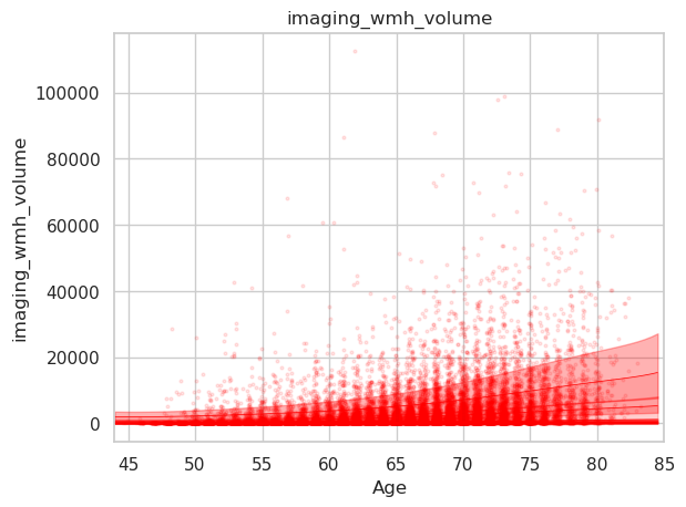
Here the plot resulting from the abovementioned code for plotting the WMH volume which appears as expected.
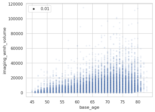
Here a simple scatterplot of the raw data.
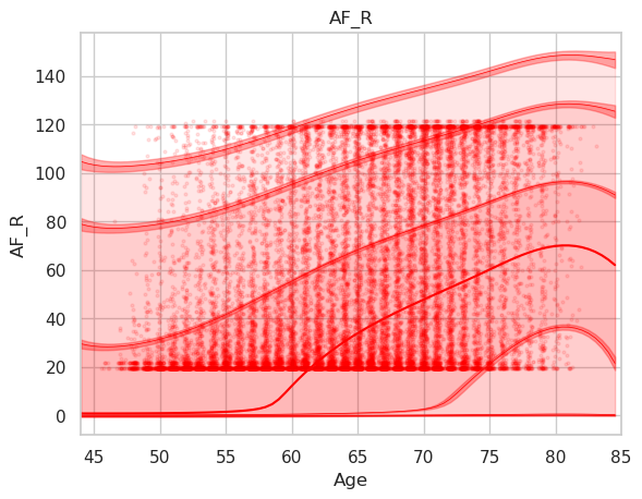
The problem is apparent when looking at other imaging-derived phenotypes.
Disconnectivity of the arcuate fascicle in percent using the abovementioned plotting code. Note that the data is shifted upwards (y interval is 20-120% instead of 0-100%).
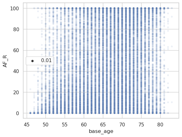
And the corresponding raw data plot.
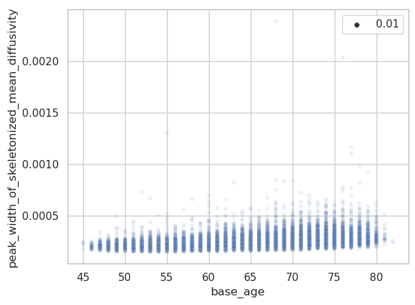
The same plots for the peak width of skeletonized mean diffusivity (PSMD).

Are there some assumptions that need to be met to apply warped BLR when modelling a variable, like is non-gaussianity of residuals required? One difference to the tutorials is that I use a 2-fold cross-validation via estimate() to get zscores for all individuals. I noticed that the resulting centile curves differ relevantly if I rerun the analysis. Maybe because of probabilistic sampling of training and test set during CV?
I would be very grateful to get some help. Happy to provide further information if required.


