Git Product home page Git Product logo

ggdist's Introduction

ggdist: Visualizations of distributions and uncertainty

R-CMD-check Coverage status CRAN status Download count Paper DOI Software DOI

ggdist is an R package that provides a flexible set of {ggplot2} geoms and stats designed especially for visualizing distributions and uncertainty. It is designed for both frequentist and Bayesian uncertainty visualization, taking the view that uncertainty visualization can be unified through the perspective of distribution visualization: for frequentist models, one visualizes confidence distributions or bootstrap distributions (see vignette("freq-uncertainty-vis")); for Bayesian models, one visualizes probability distributions (see the tidybayes package, which builds on top of {ggdist}).

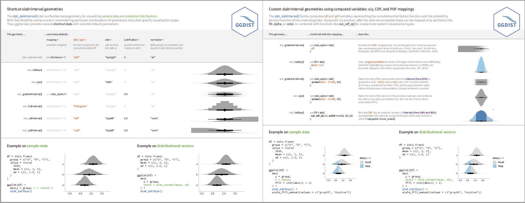
The geom_slabinterval() / stat_slabinterval() family (see vignette("slabinterval")) makes it easy to visualize point summaries and intervals, eye plots, half-eye plots, ridge plots, CCDF bar plots, gradient plots, histograms, and more:

The slabinterval family of geoms and stats

The geom_dotsinterval() / stat_dotsinterval() family (see vignette("dotsinterval")) makes it easy to visualize dot+interval plots, Wilkinson dotplots, beeswarm plots, and quantile dotplots (and combined with half-eyes, composite plots like rain cloud plots):

The geom_lineribbon() / stat_lineribbon() family (see vignette("lineribbon")) makes it easy to visualize fit lines with an arbitrary number of uncertainty bands:

All stats in {ggdist} also support visualizing analytical distributions and vectorized distribution data types like distributional objects or posterior::rvar() objects. This is particularly useful when visualizing uncertainty in frequentist models (see vignette("freq-uncertainty-vis")) or when visualizing priors in a Bayesian analysis.

The {ggdist} geoms and stats also form a core part of the tidybayes package (in fact, they originally were part of {tidybayes}). For examples of the use of {ggdist} geoms and stats for visualizing uncertainty in Bayesian models, see the vignettes in {tidybayes}, such as vignette("tidybayes", package = "tidybayes") or vignette("tidy-brms", package = "tidybayes").

Cheat sheets

These cheat sheets focus on the slabinterval family of geometries:

Installation

You can install the currently-released version from CRAN with this R command:

install.packages("ggdist")

Alternatively, you can install the latest development version from GitHub with these R commands:

install.packages("devtools")
devtools::install_github("mjskay/ggdist")

Dependencies

{ggdist} aims to have minimal additional dependencies beyond those already required by {ggplot2}. The {ggdist} dependencies fall into the following categories:

  1. {ggplot2}.

  2. Packages that {ggplot2} also depends on. These packages add no additional dependency cost because {ggplot2} already requires them: {rlang}, {cli}, {scales}, {tibble}, {vctrs}, {withr}, {gtable}, and {glue}.

  3. Packages that {ggplot2} does not depend on. These are all well-maintained packages with few dependencies and a clear need within {ggdist}:

    • {distributional}: this implementation of distribution vectors powers much of {ggdist}. This package adds minimal additional cost, as its only dependency that is not also a dependency of {ggplot2} is {numDeriv}, which is needed by {ggdist} anyway (see below).
    • {numDeriv}: used for calculating Jacobians of scale transformations. Needed because testing has revealed common situations where stats::numericDeriv() fails but {numDeriv} does not. Widely used by other CRAN packages and has no additional dependencies.
    • {quadprog}: Used to solve constrained optimization problems during different parts of dotplot layout, particularly to avoid dot overlaps in the "bin" and "weave" layouts. Widely used by other CRAN packages and has no additional dependencies.
    • {Rcpp}: Used to implement faster dotplot layout. Widely used by other CRAN packages and has no additional dependencies.

Feedback, issues, and contributions

I welcome feedback, suggestions, issues, and contributions! If you have found a bug, please file it here with minimal code to reproduce the issue. Pull requests should be filed against the dev branch. I am not particularly reliable over email, though you can try to contact me at [email protected]. A Twitter DM is more likely to elicit a response.

Citing ggdist

Matthew Kay (2024). ggdist: Visualizations of Distributions and Uncertainty in the Grammar of Graphics. IEEE Transactions on Visualization and Computer Graphics, 30(1), 414โ€“424. DOI: 10.1109/TVCG.2023.3327195.

Matthew Kay (2024). ggdist: Visualizations of Distributions and Uncertainty. R package version 3.3.2, https://mjskay.github.io/ggdist/. DOI: 10.5281/zenodo.3879620.

ggdist's People

Contributors

bwiernik avatar davidgohel avatar jtrim-ons avatar mjskay avatar paulsharpey avatar teunbrand avatar tmastny avatar

Stargazers

 avatar  avatar  avatar  avatar  avatar  avatar  avatar  avatar  avatar  avatar  avatar  avatar  avatar  avatar  avatar  avatar  avatar  avatar  avatar  avatar  avatar  avatar  avatar  avatar  avatar  avatar  avatar  avatar  avatar  avatar  avatar  avatar  avatar  avatar  avatar  avatar  avatar  avatar  avatar  avatar  avatar  avatar  avatar  avatar  avatar  avatar  avatar  avatar  avatar  avatar  avatar  avatar  avatar  avatar  avatar  avatar  avatar  avatar  avatar  avatar  avatar  avatar  avatar  avatar  avatar  avatar  avatar  avatar  avatar  avatar  avatar  avatar  avatar  avatar  avatar  avatar  avatar  avatar  avatar  avatar  avatar  avatar  avatar  avatar  avatar  avatar  avatar  avatar  avatar  avatar  avatar  avatar  avatar  avatar  avatar  avatar  avatar  avatar  avatar  avatar

Watchers

 avatar  avatar  avatar  avatar  avatar  avatar  avatar  avatar  avatar  avatar

ggdist's Issues

parse_dist() and lower bounds for class = sd

Hey @mjskay,

I wanted to use parse_dist() and stat_dist_halfeye() to compare two priors for a hierarchical $\sigma$ parameter. They were Exponential(1) and half-Normal(0, 1). With brms, the default behavior sets the lower bounds for both to zero. However, my tidybayes workflow did not set the lower bound for the half-Normal. E.g., try this:

library(brms)
library(tidybayes)
library(tidyverse)

c(prior(exponential(1), class = sd),
  prior(normal(0, 1), class = sd)) %>% 
  parse_dist(prior) %>% 
  
  ggplot(aes(y = prior, dist = .dist, args = .args)) +
  stat_dist_halfeye(.width = .95)

Attempting to manually set the lower bound with prior(normal(0, 1), class = sd, lb = 0) won't work, either. You get a warning message, instead: Error: Currently boundaries are only allowed for classe(s) 'b'.. Is there an easy fix?

Make curve_interval() work directly inside stat_lineribbon()

this is more of a questioning thing... not sure I want to re-architect treatment of the point_interval argument to stat_lineribbon() to support this since it involves making more assumptions about the type of function that can be passed there (since the function must be able to do grouping itself instead of having the grouping be done by the stat prior to calling the function). Better option might be to just add an example where use of curve_interval() with the data argument to geom_lineribbon() is shown.

support weight aes in stat_sample_slabinterval

To make everything consistent this would be a bit of a pain, so leaving it off for now. Would need to:

  • make a weighted_ecdf() function to support CDFs
  • make a weighted_quantile() function to support quantiles
  • make a weighted_hist() function to support histograms
  • make a weighted sample distribution type (.dist_weighted_sample() for now)
  • pull out weight aes and summarize sample into a .dist_weighted_sample() in compute_panel
  • pass through weight to density, weighted_ecdf, and weighted_quantile for slabs
  • use weighted histograms to support histinterval
  • add support for weights in point_interval - at least for weighted sample dist objects

Later, once support in posterior is done:

  • support weights in rvars

allow calculating all distribution functions at once in stat / stat_dist

then stick them into mappings users can use, like pdf and cdf. Would allow experimentation with even weirder custom geoms (like the Correll-style violins with faded tails)

  • stat_dist_...
  • stat_sample_...
  • fix the appearance of some NAs in the CDF calculation in stat_dist. See here: mjskay/tidybayes#136 (comment) this is due to interval data also being processed in the same geom; the fix is to set na.translate = FALSE on the fill scale. Added to examples
  • add a function for making intervals from cdfs (maybe cut_cdf_qi?)
    • re-export from tidybayes
    • add example to slabinterval vignette
  • add docs
  • add example to vignette

Should stat_dots and whatnot auto-group by numeric x/y values?

Bit of potentially unexpected behavior revealed by this twitter thread: https://twitter.com/MYMRockMama/status/1283841342779449344?s=20

Not sure but the issue might be due to groups being determined by discrete variables only, so using a numeric y value means every dot gets its own group (and so they get auto-assigned bad bin widths):

tibble(
  g = c("a","b"), 
  y = as.numeric(factor(g)) - 0.1, 
  x = list(qnorm(ppoints(100)))
) %>% 
  unnest(x) %>% 
  ggplot(aes(x = x, y = y)) + 
  stat_dots()

image

Some workarounds: (1) manually set the group aesthetic

tibble(
  g = c("a","b"), 
  y = as.numeric(factor(g)) - 0.1, 
  x = list(qnorm(ppoints(100)))
) %>% 
  unnest(x) %>% 
  ggplot(aes(x = x, y = y, group = y)) + 
  stat_dots()

image

(2) use a discrete variable for the y axis (and if you want to nudge positions do so with position_nudge:

tibble(
  g = c("a","b"), 
  x = list(qnorm(ppoints(100)))
) %>% 
  unnest(x) %>% 
  ggplot(aes(x = x, y = g)) + 
  stat_dots(position = position_nudge(y = -0.1))

image

Question is, should groups be auto-created along the x/y axis to avoid the unexpected behavior? Are there any downsides?

Further thoughts on parse_dist

Following up on this, my naive attempts fail:

library(brms)
library(tidybayes)

p <- get_prior(qsec ~ hp + (1 + hp | cyl), mtcars)
parse_dist(p)

#Error in eval_tidy(enquo(dist_col), object) : object '' not found

Although this works, but without the rest of the table (i.e. class, coef etc.):

parse_dist(p$prior)

I get the same error when asking for the parse_dist of a prior object:

p2 <- prior(normal(0, 2))
parse_dist(p2)

But a direct string version works:

parse_dist('normal(0, 2)')

I suppose my attempts fail because they are dispatching to parse_dist.data.frame, which requires you to define a prior column. So I defined a brmsprior method:

parse_dist.brmsprior <- function(object, ...) tidybayes:::parse_dist.data.frame(object, 'prior', ...)

This works for p2 above, but yields all NAs for p.

Add a fill_ramp and color_ramp aesthetics for lineribbons and slabs

Or something like that. See @mitchelloharawild's comment: #14 (comment)

Thinking about this more, it is probably useful for gradientinterval as well, since it seems the case that R graphics devices don't really support alpha gradients in the way they would need to for it to be reliable.

However, I am not sure think lightness is the right axis. I think generically allowing a color ramp from the fill to an arbitrary color (default white) in Lab space would work. Then 0 would be the other color, 1 would be the fill color, and the default limits would be set to include 0 in the input domain for continuous scales. Probably would use the same approach as alpha for discrete scales (range has lower limit 0.1).

This way, if someone wants to use a gradient with a non-white background they can do that well enough (as long as no gradients overlap, which --- well --- if someone is trying to do that there's probably a bigger problem).

Perhaps a better name then is scale_fill_ramp

  • basic impl
  • add to slabinterval
  • add to lineribbon
    • fix legend
  • tests for slabinterval
  • rewrite gradientinterval with this doesn't solve the problem anyway
  • add examples to vignettes
    • slabinterval
    • lineribbon
  • add examples to function docs
    • slabinterval

overlap from the bottom

I am summarizing multiple posteriors with stat_slab() with value on the x and key on the y. I'd like the densities to overlap a bit, say with height = 1.5 and alpha = 3/4. With this setup, it appears that the densities higher up on the y-axis overlap those on the bottom. Is is possible to reverse this behavior so that the tops of the densities lower on the y overlap the bottoms of the densities above them?

library(tidyverse)
library(tidybayes)

n <- 1e4

tibble(x = rnorm(n),
       y = rnorm(n)) %>% 
  gather() %>% 
  ggplot(aes(x = value, y = key)) +
  stat_slab(height = 1.5, color = "black", alpha = 3/4)

I get the desired behavior with ggridges::geom_density_ridges().

geom_raincloud

Any chance this might happen? I know, I know, this might be an annoying request, but.....

Add support for p boxes

Maybe:

  • vector type for p boxes (maybe put in another package)
  • stat_pbox or something like that

stat_lineribbon and multimodal distributions

Hi
I'm using stat_lineribbon with mode_hdi to plot a multimodal distribution changing with time.

It correctly plots the uncertainty in splitted intervals but it only shows a global mode. It is possible to show all the modes instead of the biggest one only? Is this functionality implemented?

thanks
FKG

improve parameter docs for slabinterval

Need some nice way of getting all the possible arguments (including from the geoms) into the documentation page of each stat/geom. Currently the multiple-chains-of-... and the stat/geom thing make it so that some args don't propagate all the way to each documentation page. Easiest thing might be to just make a template function that does this rather than trying to use the parameter inheritance stuff.

Because of #106 this is basically done except for getting geom stuff copied into the stats in a nice way. Might actually be able to handle that using param inheritance.

done for:

  • slabinterval stats
  • slabinterval geoms
  • dotsinterval stats
  • dotsinterval geoms
  • lineribbon stat

Adjust position of points/intervals on the density axis.

I'm trying to plot two interval distributions side-by-side (to show group overlap). I'd like to be able to adjust the position of the summary points/intervals so that they don't overlap each other, but I can't see a way to do that (e.g., to move one group's summary statistics up on the y-axis when the variable values are on the x-axis). Could something like point_offset and interval_offset parameters be added?

ggplot extension for 2-dimensional HPD regions

Hi there,

great package. I was wondering whether you might be interested in adding a new ggplot2 stat and geom.

I recently wanted to plot a two-dimensional HPD region for the posterior predictions of my model. Because of my bounded outcome variable, I was unhappy with the normal approximation created with stat_ellipse(). Merging emdbook::HPDregionplot() and StatContour(), I came up with the following solution based on MASS::kde2d():

#' Contours of a HDP region estimate
#'
#' @param prob Numeric. Probability level of the HDP region.
#' @inheritParams ggplot2::stat_density_2d
#' @inheritParams MASS::kde2d
#' @param ...
#'
#' @return
#' @export

stat_hpd_2d <- function(mapping = NULL, data = NULL, geom = "polygon",
                        position = "identity", na.rm = FALSE, show.legend = NA,
                        inherit.aes = TRUE, n = 100, prob = 0.95, ...) {
  ggplot2::layer(
    stat = StatHPDContour, data = data, mapping = mapping, geom = geom,
    position = position, show.legend = show.legend, inherit.aes = inherit.aes,
    params = list(na.rm = na.rm, n = n, prob = prob, ...)
  )
}

StatHPDContour <- ggplot2::ggproto(
  "hpd_2d"
  , Stat
  , compute_group = function (data, scales, na.rm = FALSE, h = NULL,
                              n = 100, prob = 0.95)
  {
    if (is.null(h)) {
      h <- c(MASS::bandwidth.nrd(data$x), MASS::bandwidth.nrd(data$y))
    }
    dens <- MASS::kde2d(data$x, data$y, h = h, n = n,
                        lims = c(scales$x$dimension(), scales$y$dimension()))
    df <- data.frame(expand.grid(x = dens$x, y = dens$y), z = as.vector(dens$z))
    df$group <- data$group[1]

    dx <- diff(dens$x[1:2])
    dy <- diff(dens$y[1:2])
    sz <- sort(dens$z)
    c1 <- cumsum(sz) * dx * dy

    breaks <- sapply(prob, function(x) {
      withCallingHandlers(
        stats::approx(c1, sz, xout = 1 - x)$y
        , warning = function(w) {
          if (grepl("collapsing to unique 'x' values", w$message))
            invokeRestart("muffleWarning")
        }
      )
    })

    ggplot2::StatContour$compute_panel(df, scales, breaks = breaks)
  }
  , required_aes = c("x", "y")
)

Here's an example:

library("ggplot2")
ggplot(data = iris, aes(x = Sepal.Length, y = Sepal.Width, color = Species)) +
    stat_hpd_2d(aes(fill = Species), prob = 0.8, alpha = 0.1, linetype = "22", size = 0.3) +
    geom_point(size = 3, alpha = 0.6)

stat_hpd

If this is something you'd be interested in, I'd be happy to expand this into a PR (add a geom, create aliases such as stat_hpd2d(), etc.). What do you think?

stat_histinterval: odd behavior for groups with no variance

If all values in a group are the same (not uncommon for a baseline or control condition), the histogram borks.
Maybe something to do with bin size?

set.seed(1234)
df = tribble(
  ~group, ~value,
  "a",    rep(10, 1000), # no variance here
  "b",    rnorm(1000, mean = -5),
  "c",    rnorm(1000, mean = 10),
) %>%
  unnest(value)

df %>%
  ggplot(aes(y = group, x = value)) +
  stat_histinterval(slab_type = "histogram") +
  theme_ggdist()

image

A workaround is to filter out the non-variant group and add it as an annotation.

Feature-request: stat_lineribbon with continuous filling

Dear reader,
it would be awesome to get the possibility of filling the stat_lineribbon with a continuous (but maybe binned) colour sclae. This way I hope to prevent the legend in vertical box theme from taking two rows when there are mor than for levels.

Sincerely, Simon

Add curve_interval()

See:
https://pubmed.ncbi.nlm.nih.gov/26356979/
https://pubmed.ncbi.nlm.nih.gov/24051838/
https://arxiv.org/abs/2007.05035

stat_dist_*() and gganimate

I understand that stat_dist_*() can not be used with gganimate because it produces a list-column.

library(dplyr)
library(ggplot2)
library(gganimate)
library(tidybayes)
p <- tribble(
   ~mean, ~sd, ~.iter,
   5,   1,      1,
   7,   1.5,    2,
   8,   1,      3,
   9,   1,      4,
   7,   1,      5
) %>%
  ggplot(aes(x = "", dist = "norm", arg1 = mean, arg2 = sd)) +
  stat_dist_eye() +
  transition_manual(.iter)

p
#> Error in mapply(FUN = f, ..., SIMPLIFY = FALSE) : 
#>   zero-length inputs cannot be mixed with those of non-zero length

Could you confirm that and, if possible, add something about it in the documentation?

Stan distribution functions

I love the new stat_dist_halfeye() function. However, I think the current approach of matching stan distribution names to existing R functions (see below) may not be ideal. In some cases, the R function differs from the stan function in argument names, orderings, and even parameterizations.

https://github.com/mjskay/tidybayes/blob/ed254b9920e8407536f3f2e5f7f4b034e85a0df3/R/parse_dist.R#L150-L167

To address this issue, I have been creating an R function for each stan distribution function that remains true to the stan function. See my progress at github.com/jmgirard/standist.

I wonder if you might consider using these functions in the lookup table above (similar to what is already being done for brms::student_t()), or permitting me to do so via PR. If you are interested, I would be open to either importing from standist or rolling this project into tidybayes.

On a related note, in that same standist repo linked above, I am working on easy single-line function calls to visualize stan distributions (for pedagogical purposes and for selecting priors). Something like viz("student_t(3, 0, 10)") or viz("student_t", arg1 = seq(1, 10, 2), arg2 = 0, arg3 = 1). I have some basic implementation of this using ggplot2::stat_function() but I think it'd be more robust and flexible to use your tidybayes::stat_dist_halfeye() function. Any interest in collaborating on this?

Consistent y-axis height for stat_dots

I love the stat_dots() slab element, especially the quantile version. But it seems to have inherited the major limitation of geom_dotplot() that the linear scale of the y-axis is meaningless.

I'm interested in combining a dots slab with a curve (e.g., to show the observed group distributions against reference normal distributions), but I'm struggling with a way to get consistent y-axis heights for the dots stacks and the density curve, especially across image sizes. See the reprex below.

Is there any way that different slab elements could be forced to use the same linear y-axis scale as the dots slab?

library(dplyr)
library(tidyr)
library(ggdist)
library(ggplot2)
library(broom)
library(modelr)

theme_set(theme_ggdist())

set.seed(5)
n = 10
n_condition = 5
ABC =
  tibble(
    condition = rep(c("A","B","C","D","E"), n),
    response = rnorm(n * 5, c(0,1,2,1,-1), 0.5)
  )
m_ABC = lm(response ~ condition, data = ABC)

ABC %>%
    data_grid(condition) %>%
    augment(m_ABC, newdata = ., se_fit = TRUE) %>%
    ggplot(aes(y = condition)) +
    stat_dist_halfeye(
        aes(dist = distributional::dist_normal(.fitted, sigma(m_ABC)))
    ) +
    # we'll add the data back in too (scale = .5 above adjusts the halfeye height so
    # that the data fit in as well)
    stat_dots(quantiles = 100, aes(x = response, y = condition), data = ABC, color = "blue")

Add stat_ribbon()

Much like stat_dist_lineribbon(), but without the line. Alternatively, stat_dist_lineribbon() could be extended to support 0 or >1 functions to allow 0 or more than 1 line.

This will be used by fabletools v0.4.0 as distributional::geom_hilo_ribbon() gets deprecated.


The motivating example for this is showing both mean and median forecasts for asymmetric distributions, such as the Log-normal distributions below.

library(fable)
#> Loading required package: fabletools
eggs <- as_tsibble(fma::eggs)
eggs %>% 
  model(ETS(log(value))) %>% 
  forecast(h = 100) %>% 
  autoplot(eggs, point_forecast = tibble::lst(mean, median))

Created on 2021-01-10 by the reprex package (v0.3.0)

interval_size_range in geom_interval has a strange interaction with the legend

Hello! Thanks for tidybayes!

I'm using interval_size_range as a way to increase the height of the interval (there's a lot of empty space on the y-axis without it), which is definitely not its intended use. However, it does have an annoying side effect of changing the size of the key in the legend.

Is there a better way to change the height/width of the interval? Or is there a way to change the legend key. I've tried to adjust legend.key.height in ggplot2::theme, but it appears to only affect the text size of each key.

Here's a reprex that demonstrates what I'm on about:

library(tidyverse)
library(tidybayes)
library(magrittr)
#> 
#> Attaching package: 'magrittr'
#> The following object is masked from 'package:purrr':
#> 
#>     set_names
#> The following object is masked from 'package:tidyr':
#> 
#>     extract
library(ggplot2)
library(scales)
#> 
#> Attaching package: 'scales'
#> The following object is masked from 'package:purrr':
#> 
#>     discard
#> The following object is masked from 'package:readr':
#> 
#>     col_factor

data(RankCorr, package = "tidybayes")

model_one_results <- RankCorr %>%
  spread_draws(u_tau[i]) %>% 
  median_qi(.width = c(.5, .8, .95, .99)) %>% 
  mutate(.model = 1) 

model_two_results <- RankCorr %>%
  spread_draws(u_tau[i]) %>% 
  mutate(u_tau = u_tau + 1) %>% 
  median_qi(.width = c(.5, .8, .95, .99)) %>% 
  mutate(.model = 2)

overall_tbl <- bind_rows(
  model_one_results,
  model_two_results
) %>% 
  mutate(.model = as.factor(.model))

ggplot(
  data = overall_tbl,
  aes(y = interaction(i, .model), x = u_tau, colour = .model)
) +
  facet_wrap(
    vars(i),
    scales = "free",
    ncol = 1
  ) +
  geom_intervalh(
    ## comment following line in/out to see the different in the width of 
    ## interval in the plot, and in the legend
    interval_size_range = c(12, 18),
    alpha = rescale(1 - overall_tbl$.width, to = c(0.1, 1))
  ) +
  scale_color_manual(
    aesthetics = "colour",
    values = c(
      "1" = "#2C7FB8",
      "2" = "#B40F20"
    )
  ) 

Created on 2020-03-10 by the reprex package (v0.3.0)

position_jitter() leads to duplication and separation of pointintervals

Attempt to jitter a default pointinterval (or any pointinterval showing multiple ranges) leads to multiple separated pointintervals for each set of observations. I believe this occurs because the multiple bounds are constructed by the layering of multiple geom_pointinterval() instances on top of one another. These are then treated as separate items to jitter by position_jitter().

Reproducible example:

library(ggplot2)
library(tidybayes)
library(tibble)
library(magrittr)

## create some data
data <- tibble(
    xs = rep(c(rnorm(1), rnorm(1)), 20),
    ys = rnorm(40),
    groups = rep(rep(1:4), 10))

## plotting gives us overplotted pointintervals
data %>% ggplot(
             aes(x = xs,
                 y = ys,
                 point_fill = factor(groups),
                 group = groups)) +
    stat_pointinterval(shape = 21) +
    scale_fill_distiller()

overplotted.pdf

## we try to jitter and this leads to duplication
jitter <- position_jitter(width = 0.1)
data %>% ggplot(
             aes(x = xs,
                 y = ys,
                 point_fill = factor(groups),
                 group = groups)) +
    stat_pointinterval(shape = 21,
                       position = jitter) +
    scale_fill_distiller()

failed_jitter.pdf

One-sided intervals

Per a request for one-sided intervals, should add them. My initial thought is that the obvious way to add them is via a new interval type in the point_interval family, so that .width and such can continue to be used and everything else will just work fine (TM). By analogy to current naming scheme (qi / hdi) should be something like loweri / upperi or li / ui or lowi / highi or lefti / righti or ll / ul or lowerl / upperl. Not sold on any of the names yet.

Changes would need to be:

  • add the interval functions
  • add the mean_/median_/mode_ + interval functions
  • figure out how to support these in stat_dist_..., which might involve adding a point_interval argument there that takes character vectors in the pattern of point_interval functions in stat_sample_.... Would also want to double-check stat_sample... does match.fun on character vector args for consistency across the two sub-families. (This would simultaneously solve the problem of using something other than median on distributions: could call down to the mean function for {distributional} objects for example if the mean is requested in analytical distributions). Or could add implementations of qi/hdi for distributional objects, which would simplify making point_interval implementation for them.

cut_cdf_qi is missing

Hi,

I'm trying to use cut_cdf_qi() function as in the cheatsheet, but it's not available. Neither after loading ggdist through library(ggdist), nor through ggdist::cut_cdf_qi() nor through ggdist:::cut_cdf_qi(). And there is no help page for that function...
I've installed ggdist using install.packages("ggdist") (it's version 2.3.0). Tried to reinstall through devtools::install_github("mjskay/ggdist"), but it gets stuck forever on downloading.

Do you know, what could be the problem? Thanks in advance!
Evgeny

> sessionInfo()
R version 4.0.0 (2020-04-24)
Platform: x86_64-apple-darwin17.0 (64-bit)
Running under: macOS Catalina 10.15.7

Matrix products: default
BLAS:   /System/Library/Frameworks/Accelerate.framework/Versions/A/Frameworks/vecLib.framework/Versions/A/libBLAS.dylib
LAPACK: /Library/Frameworks/R.framework/Versions/4.0/Resources/lib/libRlapack.dylib

locale:
[1] en_US.UTF-8/en_US.UTF-8/en_US.UTF-8/C/en_US.UTF-8/en_US.UTF-8

attached base packages:
[1] stats     graphics  grDevices utils     datasets  methods   base     

other attached packages:
[1] ggdist_2.3.0

loaded via a namespace (and not attached):
 [1] Rcpp_1.0.5           rstudioapi_0.13      magrittr_2.0.1       tidyselect_1.1.0    
 [5] munsell_0.5.0        colorspace_2.0-0     R6_2.5.0             rlang_0.4.9         
 [9] fansi_0.4.1          dplyr_1.0.2          tools_4.0.0          grid_4.0.0          
[13] packrat_0.5.0        gtable_0.3.0         cli_2.2.0            ellipsis_0.3.1      
[17] assertthat_0.2.1     tibble_3.0.4         lifecycle_0.2.0      crayon_1.3.4.9000   
[21] tidyr_1.0.2          farver_2.0.3         purrr_0.3.4          ggplot2_3.3.2       
[25] vctrs_0.3.5          glue_1.4.2           compiler_4.0.0       pillar_1.4.7        
[29] forcats_0.5.0        generics_0.0.2       scales_1.1.1         distributional_0.2.1
[33] pkgconfig_2.0.3  

Next CRAN release

(this issue is never closed, just re-used for the next release)

  • check for existing problems on CRAN checks for ggdist
  • double-check CRAN policies
  • check package for large files: output from devtools::build() is less than 5MB
  • remove any Remotes in DESCRIPTION and downgrade those packages back to CRAN versions
  • update R and all packages
    • devtools::install_dev_deps()
    • update.packages(ask = FALSE)
  • bump version and date
    • in DESCRIPTION
    • in NEWS
  • devtools::check(remote = TRUE, manual = TRUE)
  • check tests on {tidybayes} manually
  • revdepcheck::revdep_check(num_workers = 6)
    • if any packages time out, add them back with revdep_add() then run with a large timeout, e.g. revdepcheck::revdep_check(num_workers = 6, timeout = as.difftime(500, units = "mins"))
  • update NEWS
  • spelling::spell_check_package()
    • spelling::update_wordlist()
  • urlchecker::url_check()
    • on failures, urlchecker::url_update()
  • lintr::lint_package()
  • devtools::document()
  • devtools::install()
  • rebuild README
  • pkgdown::clean_site()
  • pkgdown::build_site(run_dont_run = TRUE)
  • devtools::check(remote = TRUE, manual = TRUE)
    • R-release, on Windows
    • Whatever platforms on Github actions
  • devtools::check_win_release()
  • devtools::check_win_devel()
  • devtools::check_win_oldrelease()
  • write cran-comments.md
  • devtools::release()

After package goes live on CRAN:

  • merge dev onto master and cran
  • tag release
  • double check zenodo entry
    • authors
    • license (GPL >= 3)
    • title (ggdist: Visualizations of distributions and uncertainty)
    • NSF award 2126598
    • related VIS paper: is published in 10.1109/TVCG.2023.3327195
  • revdepcheck::revdep_reset()
  • bump to a new dev version on dev branch
  • skeet

Template loosely based on r-lib/usethis#338

Recommend Projects

  • React photo React

    A declarative, efficient, and flexible JavaScript library for building user interfaces.

  • Vue.js photo Vue.js

    ๐Ÿ–– Vue.js is a progressive, incrementally-adoptable JavaScript framework for building UI on the web.

  • Typescript photo Typescript

    TypeScript is a superset of JavaScript that compiles to clean JavaScript output.

  • TensorFlow photo TensorFlow

    An Open Source Machine Learning Framework for Everyone

  • Django photo Django

    The Web framework for perfectionists with deadlines.

  • D3 photo D3

    Bring data to life with SVG, Canvas and HTML. ๐Ÿ“Š๐Ÿ“ˆ๐ŸŽ‰

Recommend Topics

  • javascript

    JavaScript (JS) is a lightweight interpreted programming language with first-class functions.

  • web

    Some thing interesting about web. New door for the world.

  • server

    A server is a program made to process requests and deliver data to clients.

  • Machine learning

    Machine learning is a way of modeling and interpreting data that allows a piece of software to respond intelligently.

  • Game

    Some thing interesting about game, make everyone happy.

Recommend Org

  • Facebook photo Facebook

    We are working to build community through open source technology. NB: members must have two-factor auth.

  • Microsoft photo Microsoft

    Open source projects and samples from Microsoft.

  • Google photo Google

    Google โค๏ธ Open Source for everyone.

  • D3 photo D3

    Data-Driven Documents codes.