Simulation software of an agent-based multiscale model for a population of communicating cells. This guide provides instructions for installation and utilisation of the application. The software consists of a program with GUI that allows users to simulate and analyse our model without writing code, and comes with various input/output features to store and load simulation data. It is available both for MATLAB users and users without MATLAB. MATLAB users can install MultiCellSim as an app and directly run it from the Apps tab. Non-MATLAB users can download a standalone executable file that installs MATLAB Runtime (no licence required) in addition to MultiCellSim. Our goal here is to provide an open-source simulation software of the model, which anyone can use and modify for research or educational purposes (see Licence for details).

How do communicating cells self-organize into complex spatiotemporal patterns? We modelled cells that secrete and sense the same set of signalling molecules as a discrete dynamical system. Through tuning molecular parameters such as the secretion rate and response of the cells and the effective distance between cells we observed a rich palette of self-organized patterns, ranging from static islands to collective oscillations and travelling waves. For cells communicating with one signalling molecule, we were able to identify various phases, in some of which cells behave autonomously whereas in others they behave collectively (Maire & Youk, 2015). The collective dynamics of the system is effectively described by an pseudo-energy, where we can picture a ball rolling down a landscape shaped by two macroscopic parameters of the system (Olimpio, Dang & Youk, 2018). The extension to two molecules revealed a surprising variety of dynamic patterns such as oscillations and travelling waves, which we could analyse and predict through an analytic framework we developed (Dang, Grundel & Youk, 2020).

More information on the model and research can be found here. The papers in which the model was first published and further developed are:

• T. Maire and H. Youk. Molecular-level tuning of cellular autonomy controls collective behaviors of cell populations. Cell Systems 1, 349–360 (2015).
• E. P. Olimpio*, Y. Dang*, and H. Youk. Statistical dynamics of spatial-order formation by communicating cells. iScience 2: 27-40 (2018).
• Y. Dang, D. Grundel and H. Youk, Cellular Dialogues that enable self-organization of dynamic spatial patterns, Cell Systems 10, 82-98 (2020)

To cite MultiCellSim, please cite the Dang et al. paper, as the software was developed as part of this publication. Additional ideas and background for this project can be found on the Wiki page.

Full source code of all scripts used to generate the data in the Dang et al. paper is available in another GitHub repository.

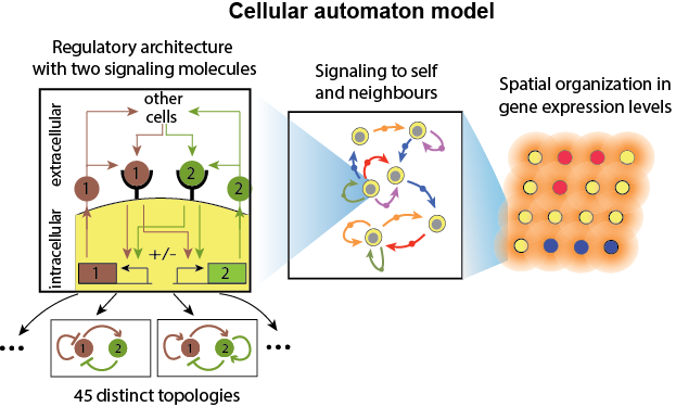
Schematic of the model underlying the simulation app.

Example of self-organized pattern observed in a simulation. Snapshots following each other may be separated by different number of time steps.

Please go to the Releases page to download the latest release of MultiCellSim to follow the instructions below. Alternatively, you can download or clone the entire repository or a subset of it and install MultiCellSim manually.

MATLAB (R2019a). Earlier versions of MATLAB from R2016b onwards should also work, but we recommend manual installation (see below).

Using the App Installer:

1. Download the .mlappinstall file of the latest release.
2. Run the MATLAB Installer file. The program should unpack itself and install as an app in MATLAB.
3. Run the installed app "MultiCellSim" from the "Apps" menu in MATLAB.

Manually (recommended for MATLAB versions before R2018b):

1. Download the source files from the release.
2. Move the content to a location in which you have write permission (to store files). Also, make sure the folder is empty to prevent possible conflicts when running the code.
3. Run the .mlapp file compatible with your MATLAB version to directly run the app.

It is possible to install and run the full simulation software without installing MATLAB. Instead, the user can simply run executable program that downloads and installs MATLAB Runtime in addition to the application MultiCellSim.

1GB of storage, administrator rights on your PC and a working Internet connection.

1. Download the zipped installer from the latest release and unzip the file.
2. Run the installer (.exe file for Windows, .app file for macOS). You will first be prompted to choose the installation folder for the software (default location: C:\Program Files\TU Delft\MultiCellSim) and then for MATLAB Runtime in case you have not installed it before (default location: C:\Program Files\MATLAB\MATLAB Runtime).
3. The installer will download and install the files for MATLAB Runtime R2019 (no licence required) before installing MultiCellSim. Note that the installation of MATLAB Runtime may take a considerable time due to its size (~786MB in total).
4. Run the program MultiCellSim. It may take a while to boot. In the meantime, you will be entertained with a snapshot from a simulation. Note: as the installation program is an executable file, your PC might consider it unsafe and pass is through your virus scanner first.

Uninstall MultiCellSim as you would uninstall any other program on your Windows or macOS PC. In Windows, go to Control Panel > Programs > Programs and Features, select MultiCellSim and click Uninstall. Alternatively, you can manually run the uninstall executable program. First go to the folder in which the software is installed (default: C:\Program Files\TU Delft\MultiCellSim). Go to the subfolder ~\uninstall\bin\win64 (or win32 depending on your PC) and run uninstall.exe. Note that uninstalling MultiCellSim does not automatically uninstall MATLAB Runtime.

The GUI consists of (A) a menu at the top, (B) a left box with tabs for simulating with one and two molecules, with editable fields and switches under each tab, (C) a figure displaying the cellular lattice, (D) buttons for simulation control, (E) options for randomizing cell positions, (F) options for moving cells, (G) options for modifying the logic gate specifying how the signals should be combined, (H) buttons for switching between different signal displays, (I) a toggle bar for controlling the speed of the simulation and (J) a message box for output messages. Let's go through the components one by one.

Overview of the GUI.

For one signal, the parameters tab is simpler.

Direct visualisation of the multicellular system is presented in the central box. The circles represent the cells and the color their expression level.

In the case of one signalling molecule, the expression levels are plotted on a grayscale, with darker colors corresponds to a higher expression levels. For the binary system, OFF cells are white and ON cells are black. In the continuous system, the darker of the shade of grey, the higher the expression level of the cell. The color bar on the right shows how the colors match to the exact states of the cells.

Color legend for gene expression of a single gene. Darker colors represent higher relative gene expression level (0 = lowest level, 1 = highest level). For two signals, a similar legend can be made in the app (see below).

In the case of two signalling molecules, we display the level of the two molecules using yellow and blue colors. Yellow corresponds to gene 1 and blue corresponds to gene 2. Hence for the binary system,

• A white cell corresponds to the state (0,0), where both genes are off.
• A red cell corresponds to the state (1,0), where only gene 1 is on.
• A blue cell corresponds to the state (0,1), where only gene 2 is on.
• A black cell corresponds to the state (1,1), where both genes are on.

The caption above the figure displays the time (in units of time steps) and statistics of the current figure. Here, p is the mean expression level of the cells and I (optionally displayed) is a spatial index measuring the degree of spatial organisation of the cells (see the Olimpio et al. paper). In short, if I=0 the system is fully disordered whereas for |I|->1 the system becomes spatially ordered. For cells with continuous gene expression, the degree of redness and degree of blueness represent the degree to which genes 1 and 2 are expressed respectively.

The controls for running the simulation are based on media playback buttons (panel D). Click on the "PLAY" button to run a new simulation. The "PAUSE" button will pause the simulation and resume once you press "PLAY" again. The simulation continues until the system reaches equilibrium (when none of the cells changes state upon updating), or when the maximum simulation time is reached (by default set to tmax = 10^6). To stop a current simulation or reset a terminated simulation, press the "STOP" button. This erases the current simulation and all data associated with it, so if you intend to save the simulation, do so before you press "STOP".

The four buttons at the bottom are for going through a simulation without running it for more time (Replay mode). The skip forward and backward buttons skip to the start and end of the current simulation. The seek forward and backward buttons move the simulation by one step in time. At any time, the simulation can be run again by pressing "PLAY". If the simulation did not reach equilibrium, it will continue running after the last frame of the replay has been reached. In the "Simulation" menu, there is an additional option "Skip to time" that allows you to directly skip to a time you input.

Finally, the "Simulation speed" slider (panel I) controls the speed of the simulation or playback (i.e. how fast the frames follow each other).

For two types of signals, we can plot both at the same time, or focus on one of the two. The "Display signal" button group allows you to toggle between these different views of the cells. Selecting "1" will display the level of gene 1 on a grayscale, "2" displays gene 2 and "both" displays both genes using the color scheme described above.

There are two tabs to switch between cells that communicate with one signaling molecule and cells that communicate with two molecules.

The first tab is for simulating a system where the cells communicate through one type of signalling molecule. Detailed descriptions of the variables can be found in the papers listed above. Below is a quick overview of all parameters of the system.

• Interaction. This allows you to toggle between activating and repressive interaction of the single molecule.
• Cell Size. The cell size is the radius of the cell in units of a0 (see below). It's maximum value is 1/2, which correpsonds to the case where nearest-neighbor cells are touching.
• Grid size. Sets the size of the lattice. The constructed lattice will be a triangular lattice with both size consisting of 'grid size' number of cells.
• a0. Effective distance between the cells. This sets the interaction strength between the cells. A small value of a0 corresponds to strongly interacting cells, whereas for large a0 cells have little influence on each other.
• K. Sensing threshold. In the binary system with activating interaction, this sets the threshold for the concentration cells must sense to turn ON. In the continuous system, this is the sensed concentration at which the cells are exactly halfway between their lowest and highest expression levels.
• Con. Maximum secretion rate. This is the secretion rate attained by ON cells in the binary system, or the maximum secretion rate in the continuous system.
• Noise. Stochasticity is modelled as a stochastic term in the sensing threshold K. The value of this field sets the strength of the fluctuations of K. Specifically, we model the noise as an additive normally distributed stochastic variable and the noise coefficient sets the width (standard deviation) of the Gaussian in units of K.
• Hill coefficient. Sets the steepness of the response function. A high Hill coefficient corresponds to a sharp response around the value of K, whereas a low value corresponds to a gradual response. By default, it it set to 'Inf' to simulate the binary system.
• p(t=0). Initial mean expression level of the system (values between 0 and 1). In the binary system, this corresponds to the initial fraction of ON cells.
• I(t=0). Initial spatial index of the system (values between -1 and 1). A value of 0 corresponds to a random distribution of cell states across space, whereas a value close to 1 (-1) corresponds to cell states that are positively (negatively) correlated with each other in space. In order to use this function, the user must first select "Initiate with I(t=0)" from the Options menu. Otherwise, the system will be initiated without constraints on the initial spatial index.

This tab is for simulating cells that communicate through two types of signalling molecule, which we assume do not directly interfere with each other. However, both are able to influence the state of the cell, and can do so in different ways. This tab is for simulating multiplicative interactions, where the effects to the the two signaling molecules multiply. This corresponds to an AND logic gate in the case of step-function responses. Biophysically, multiplicative interactions can happen when there is a gene with multiple promoters, that requires activators to be bound to all promoters before the gene is transcribed. Concretely, an example of multiplicative interaction is a cell that upregulates its expression of gene 1 only if it senses a high concentration of both signal 1 and signal 2. If one of the two has a low level, the cell will not upregulate its expression level.

In this case, there is a number of changes in the parameters that describe the system:

• lambda12. This is the ratio between the diffusion length of the two signalling molecules. The diffusion length sets a typical length scale for the decay of the signalling molecule surrounding a given cell. All lengths in the system are expressed with respect to lambda1, the diffusion length of molecule 1.
• K = K_ij. Instead of a having a single threshold K (for infinite Hill coefficient), we now have a threshold for each interaction of the system. With two molecules, there are four interactions. The noise term is still in units of the thresholds (see above), so we have a different normalisation for each noise term.
• Con = Con_i. Likewise, the two signalling molecules can have different maximum production rates. In addition, there is also the 'OFF' production rate for each gene, Coff_i, which can be different from each other. For simplicity, however, we set Coff_i=1 for all genes.
• p1(t=0), p2(t=0). We define a mean expression level for each of the two genes. As initial condition we can then set the average gene expression for both genes.
• I1(t=0), I2(t=0). Likewise, we define spatial indices for both types of molecules. The two spatial indices are independent of each other for any fixed configuration of the system. In order to use this function, the user must first select "Initiate with I(t=0)" from the Options menu. Otherwise, the system will be initiated without constraints on the initial spatial index.

The menu on top has a number of options that are useful for plotting results, importing and exporting data and tuning settings of the simulations.

This menu contains the I/O controls as well as controls for closing windows.

• Save trajectory. Saves a simulation trajectory as a '.mat' file. The simulation data is stored as a cell array 'CellsHist' that contains the state of the cell at each time step.
• Open trajectory. Opens a saved trajectory for replaying. The opened trajectory will stay in memory until the "STOP" (reset) button is pushed or a change is made to the parameter tabs.
• Save figures. Saves all opened plots as '.pdf' or '.eps' files. The user is prompted to select the format and to confirm the name for each plot.
• Save movie. Saves the current trajectory as a video. The user is prompted to specify the range of timesteps to include in the movie, and the format of the movie (from a list of default formats for saving movies using MATLAB).
• Save system state. Allows the user to save a snapshot of the trajectory as '.xls' file for later use. The snapshot can be reloaded as initial state by selecting "Manually input initial state" under "Options" (see below). Upon selecting, the user is prompted to input the time of the snapshot to be saved.
• Close all figures. Closes all plots generated by the user.
• Close app. Closes all figures and close the app. It is recommended that you close the app in this way, because closing it by pressing the close button will not close all figures.

This contains the same controls as the buttons (described under 'Running the simulation') below the figure. It also shows the shortcuts that can be used in place of pressing the buttons.

Here you can find options to plot various properties of the running simulation. This only works if you have run or loaded a simulation and have not pressed the STOP button.

• Kymograph. Plots a kymograph or space-time plot of the dynamics. This is useful for quickly getting an overall picture of what is happening in the system.
• Mean gene expression p(t). Plots a trajectory of the mean gene expression against time. If there are two signals, the plot will contain two lines on the same plot.
• Population fractions pij(t) (binary). Plots a trajectory of the relative fractions pij(t) of the cells in state (i,j). Works only for two signals with infinite Hill coefficient.
• Spatial auto-correlation I(t). Plots a trajectory of the spatial index / auto-correlation over time.
• Spatial auto-correlation Theta(t). Same as above, but now for Theta(t) (normalized with respect to the signalling strength fN).
• Spatial cross-correlation. Plots local cross-correlations between the two genes in the system with two molecules. Distances can be either the Hamming distance or Jacard distance between the two sets of gene expression values for each of the cells of each of the genes.
• 2D trajectory (p(t),I(t)). Plots a trajectory in the (p,I) plane. The starting points are marked by coloured circles, while the endpoints are marked by circles with a cross. If there are two signals, both trajectories will be plotted.
• 2D trajectory (p(t),Theta(t)). See above, for (p,Theta/fN).
• Pseudo-energy h(t) Plots the pseudo-energy h(t) (see the Olimpio et al. paper). Only for 1 signal with binary cell states.

This contains a few optional features for running and displaying the simulations.

• Show I. Selecting this option will display the value of I on top of the figure. This might cause the simulation to run slightly slower.
• Initiate with I(t=0) (only for binary cells). Use the value of I(t=0) - or I1(t=0) and I2(t=0) in case of two signals - for the initial state. If unchecked (default), the system will generate an initial lattice by randomly selecting ON cells according to the value of p(t=0), without regard to the initial spatial order. This typically gives a value for I of around zero, but to be precise (up to 0.01), choose this option. The simulation will then run an algorithm to try to generate a lattice with the input I(t=0). As this is not always possible, the messages will display whether the outcome has been achieved or not. Note that for very high I, this can be a slow process.
• Manually input initial state. This allows the user to run a simulation from a user-specified initial state rather than a randomly generated initial state. If selected, the next time the user runs a new simulation, s/he will be prompted to manually input an excel file with the initial state (see below, "Format manual input initial state").
• Set default load folder. Allows the user to specify the default folder that pops up when "Load trajectory" (File Menu) is selected.
• Set default save folder. Allows the user to specify the default folder that pops up when any of the saving functions of the File Menu is selected.

For manually inputting cell states, the user should prepare an excel file with the gene expression levels of all the cells of the system (values between 0 and 1 for each cell). The format of the data can be of the same form as the format of the "cells" variable inside the app (i.e. a Nxl matrix where N="grid size"^2 is the number of cells and l is the number of signalling molecules). However, the user can also input files in a form that is more intuitive given the form of the lattice. For this, specify the cell states in a "grid size" times "grid size" matrix. If there are two molecules, use the first two sheets of the excel file to specify the expression levels of the two different genes. The grid size of the simulation must be set to the same value as that of the loaded excel file to be a valid input.

The controls under this menu allow you to examine certain features of the chosen parameter set.

• Circuit topology. This plots the gene circuit under consideration (according to the settings in the selected parameters tab). Blue arrows show activating interactions, red arrows show inhibiting interactions.
• Phase diagram. The phase diagram shows the "phase" of each interaction of the system. The plot is separated into two subplots for each of the signalling molecules. The markers (circles and triangles) show the values of the K and C_ON for a particular interaction. The number next to the marker indicates the gene that the signalling molecule controls. Circles are for activating interactions, triangles for repressive interactions. As a concrete example, a triangle in the lower figure with the number 1 indicates phase and the interaction parameters for a repressive interaction of molecule 2 on gene 1.
• State diagram - single cell. The state diagram shows all allowed transitions between the different states of a cell. In other words, it shows which states a cell can adopt at the next time step given its current state. For one molecule there are two states (0 and 1), for two molecules there are four ((0,0), (0,1), (1,0), (1,1)). The single cell state diagram shows the (deterministic) transitions for each of these states. For instance, an arrow between (0,0) and (1,1) means that a single cell with both genes off will always turn on both genes at the next time step. The diagrams depend on the set of parameters specified in the parameters tab.
• State diagram - full system. For the full system with N>=1 cells, the state diagram shows all possible transitions for any cell in the lattice. Transitions are no longer necessarily deterministic, so certain states can transition to multiple states depending on the states of its neighbours. For instance, a diagram with the (0,0) state linked to both (0,0) and (1,0) indicates that (0,0) cells can transition to either of the two states, depending on the signals they receive from other cells of the lattice.
• Cell color legend. This generates a legend displaying the correspondence between the colours of the simulation and the gene expression levels of the cells.
• Periodicity test. We devised a test to check if simulation has settled into a periodic motion (where the same limited set of states repeats itself). Clicking on "periodicity test" will run the test and display its results in the "Messages" box.

• Documentation. Opens the GitHub page for the app.

There are a number of additional options for modifying aspects of the simulations we shall discuss below. These correspond to extensions of the original model that can be studied to see how findings change as a number of model assumptions is altered. The details of the implementation can be found in Dang et al., 2019.

The first extended option is to randomize the positions of the cell, such that they do not sit perfectly on top of a regular hexagonal lattice. To do this, we utilized a Monte Carlo algorithm from the study of hard spheres in statistical physics to randomize the cell locations. The "degree of randomness" is determined by the number of Monte Carlo steps you let the algorithm run for. Generally, we do not recommend going to too high numbers or the algorithm might not finish in any reasonable time. In addition, the user can tune the size of the cells, which has an actual effect on the dynamics rather than being for display purposes only. If the size of the cells becomes large, the user should limit the number of Monte Carlo steps to take.

We can also let the cell move dynamically over time, so that each cell moves to a slightly different position at each time step. We implement cell motility by simultaneously updating all cell positions using random walk statistics at each time step, with the constraint that areas of the cells cannot overlap. The motility of the cells is controlled by a parameter Sigma_D, which can be tuned to let the cells move around more or move around less.

The two signals that a cell perceives can be integrated into a single response in different ways. For binary cells, the response of two binary input signals (specifying whether each sensed concentration is above or below the corresponding threshold) is a single binary variable, so the signal integration can be described by a single logic gate. Here, we consider the AND gate (both signals have to match a given criterion) and the OR gate (at least one of the signals has to match a criterion).

The message box displays messages to guide the user during the simulation. In particular, if certain steps take a long time the app might temporarily freeze, but the message box should display the task which is causing the slowdown.

A list of known issues can be found under the issues page (https://github.com/YitengDang/Multicellularity/issues). In general, if the simulation gets stuck, try pressing the "STOP" (reset) button to see if it resolves the problem. Restarting the app sometimes also does magic. If you are running the app on a laptop, the responses to user input can be slow and the simulation might not run smoothly. Note also that the app needs to be able to save data to your folders to run. If you installed using the installation package, the folder is likely the default folder in which MATLAB stores apps. If you installed manually, choose a folder where you have write permission to deploy the app. Feel free to report any other issues you find on the issues page.

MIT Licence