The dataset used for training was obtained from London Meteorological data. I have prepared the data in the excel sheet and read it in the matrix form in MATLAB. There were many features from in the data and I needed to choose the relevant data for training. The features like temperature and average temperature over a particular period were important features. I excluded features like wind direction and gust because those features have minimal correlation with the wind speed. Another important feature which was not present in the data but I added was the month of the data because season has significant impact on wind speed. Finally all the features were integrated in the excel sheet and read from MATLAB.

The dataset that I have used has 5 features as input. The neural network is generated using the “fitnet” function. In our code, the fitnet function trains a neural network which has two hidden layers along with the input and output layers. The first layer of the network has 5 neurons and it acts as the input layer with the vectors of sample data being given to it. Two hidden layers are introduced with 10 and 5 neurons each to enable the network to learn complex mathematical relationship in the dataset. I have used LM back propagation method for training.

The Levenberg-Marquardt algorithm, also known as the damped least-squares method, has been designed to work specifically with loss functions which take the form of a sum of squared errors.

Consider a loss function which can be expressed as a sum of squared errors of the form

f = ∑ e i 2 ,   i=0,...,m

Here m is the number of instances in the data set.

We can define the Jacobian matrix of the loss function as that containing the derivatives of the errors with respect to the parameters,

J i,j f(w) = de i /dw j (i = 1,...,m & j = 1,...,n)

Where m is the number of instances in the data set and n is the number of parameters in the neural network. Note that the size of the Jacobian matrix is m·n. The gradient vector of the loss function can be computed as:

ᐁf = 2 J T ·e

Here e is the vector of all error terms.

Finally, we can approximate the Hessian matrix with the following expression.

Hf ≈ 2 J T ·J + λI

Where λ is a damping factor that ensures the positiveness of the Hessian and I is the identity matrix.

The next expression defines the parameters improvement process with the Levenberg- Marquardt algorithm.

w i+1 = w i - (J i T ·J i +λ i I) -1 ·(2 J i T ·e i ),   i=0,1,...

When the damping parameter λ is zero, this is just Newton's method, using the approximate Hessian matrix. On the other hand, when λ is large, this becomes gradient descent with a small training rate.

The parameter λ is initialized to be large so that first updates are small steps in the gradient descent direction. If any iteration happens to result in a failure, then λ is increased by some factor. Otherwise, as the loss decreases, λ is decreased, so that the Levenberg-Marquardt algorithm approaches the Newton method. This process typically accelerates the convergence to the minimum.

The picture below represents a state diagram for the training process of a neural network with the Levenberg-Marquardt algorithm. The first step is to calculate the loss, the gradient and the Hessian approximation. Then the damping parameter is adjusted so as to reduce the loss at each iteration.

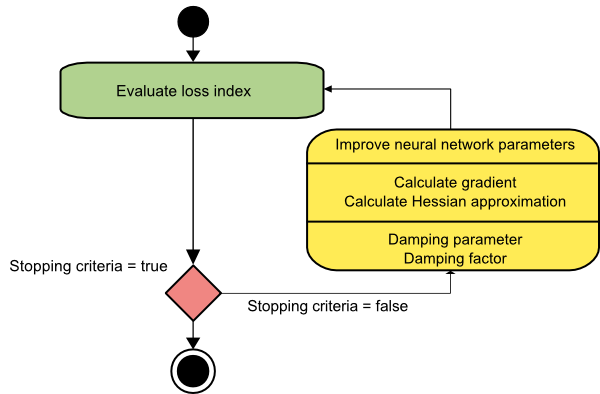
As we have seen the Levenberg-Marquardt algorithm is a method tailored for functions of the type sum-of- squared-error. That makes it to be very fast when training neural networks measured on that kind of errors.

The dataset that I used was split into Train, Validation and Test sets as follows: 70% is used for training, 15% for validation and 15% for testing. The matrix of the dataset is then sent for training using the MATLAB ‘train’ function which uses the above mentioned Levenberg- Marquardt algorithm. To reduce the error, I tried many different things and changed the hyper-parameters to reach the accuracy of 99% on the Validation and Test splits.

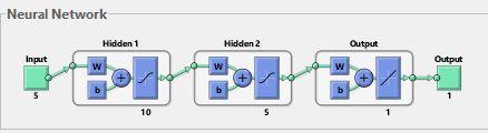
Fig 1. Neural Network model defintion

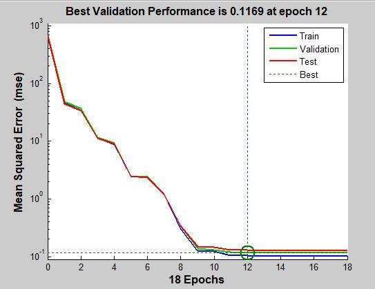
Fig 2. Performance (Mean Squared Error)

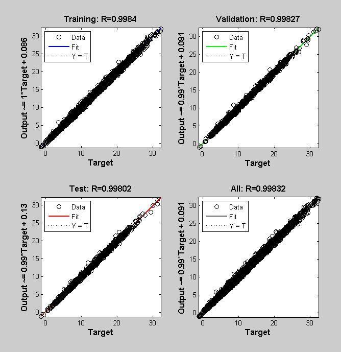
Fig 3. Training, Validation and Testing Curve

After training, the model can be used on new data by feed-forwarding the network and predicting the output as wind speed.