umit / spark-workshop Goto Github PK

Dean Wampler, Ph.D. Typesafe [email protected] @deanwampler

This workshop demonstrates how to write and run Apache Spark version 1.3 applications. You can run the examples and exercises locally on a workstation, on Hadoop (which could also be on your workstation), or both.

If you are most interested in using Spark with Hadoop, the Hadoop vendors have preconfigured, virtual machine "sandboxes" with Spark included. See their websites for information.

For more advanced Spark training and services from Typesafe, please visit typesafe.com/reactive-big-data.

You can work through the examples and exercises on a local workstation, so-called local mode. If you have Hadoop version 2 (YARN based) installation available, including a virtual machine "sandbox" from one of the Hadoop vendors, you can also run most of the examples in that environment. I'll refer to this arrangement as Hadoop mode.

Let's discuss setup for local mode first.

Working in local mode makes it easy to edit, test, run, and debug applications quickly. Then, running them in Hadoop provides more real-world testing.

We will build and run the examples and exercises using Typesafe Activator, which includes web-based and command-line interfaces. Activator includes a build tool for Scala that we'll use to download the libraries we need and to build our examples.

Activator is part of the Typesafe Reactive Platform. It is a web-based environment for finding and using example templates for many different JVM-based toolkits and example applications. Once you've loaded one or more templates, you can browse and build the code, then run the tests and the application itself. This Spark Workshop is one example.

Activator also includes SBT, which the UI uses under the hood. You can use the shell mode explicitly if you prefer running sbt "tasks".

You'll need either Activator or SBT installed. We recommend Activator.

If you are not already viewing this workshop in Activator, install it by following the instructions on the get started page. After installing it, add the installation directory to your PATH or define the environment variable ACTIVATOR_HOME (MacOS, Linux, or Cygwin only).

NOTE: Activator version 1.3 or later is required.

If you prefer SBT and you need to install it, follow the instructions on the download page. SBT puts itself on your path. However, if you have a custom installation that isn't on your path, define the environment variable SBT_HOME (MacOS, Linux, or Cygwin only).

NOTE: If you are here to learn Spark, you don't need to setup these exercises for Hadoop execution. Come back to these instructions when you're ready to try working with Spark on Hadoop. Also, this "mode" is not as well tested as I would like, so please report bugs!

If you want to run the examples on Hadoop, choose one of the following options.

The Hadoop vendors all provide virtual machine "sandboxes" that you can load into VMWare, VirtualBox, and other virtualization environments. Most of them now bundle Spark. Check the vendor's documentation.

If you have a Hadoop cluster installation or a "vanilla" virtual machine sandbox, verify if Spark is already installed. For example, log into a cluster node, edge node, or the sandbox and try running spark-shell. If it's not found, then assume that Spark is not installed. Your Hadoop vendor's web site should have information on installing and using Spark. In most cases, it will be as simple as downloading an appropriate Spark build from the Spark download page. Select the distribution built for your Hadoop distribution.

Assuming you don't have administration rights, it's sufficient to expand the archive in your home directory on the cluster node or edge node you intend to use, or within the sandbox. Then add the bin directory under the Spark installation directory to your PATH or define the environment variable SPARK_HOME to match the installation directory, not the bin directory.

You'll need to copy this workshop to the same server or sandbox. Copy the data to HDFS using the following command, which copies the workshop's data directory to /user/$USER/data:

hadoop fs -put data data

If you want to put the data directory somewhere else, you can, but you'll need to always specify that input location when you run the examples in Hadoop.

You'll also need Activator or SBT on the server or sandbox to run the examples. Recall that I recommend going through the workshop on your local workstation first, then move everything to the cluster node or sandbox to try running the examples in Hadoop.

From now on, except where noted, the instructions apply for both your local workstation and Hadoop setup.

First, change to the root directory for this workshop.

If you prefer a command-line interface, either run activator shell or sbt, depending on which tool you installed.

To use Activator's UI, run activator ui, assuming it's in your path, or use the fully-qualified path to it. It will start Activator and open the web-based UI in your browser automatically. (If not, open localhost:8888 in your browser.)

If you are trying the workshop on a Hadoop cluster or edge node, or in a sandbox, change to the workshop root directory and run the command ./start.sh. It will start Activator and load this workshop.

By default, it will start the Activator web-based UI, but you'll have to open your browser to the correct URL yourself, since you'll view the UI on a different machine, i.e., your workstation. The script prints a message to the login console showing the correct URL, including a different port number, 9999, than above. (A different port is used because 8888 is sometimes used for other purposes in Hadoop clusters.)

There are options for running in Activator shell mode or using SBT. Use ./start.sh --help to see those options.

To ensure that the basic environment is working, compile the code and run the tests; use the Activator UI's test link or the shell/sbt command test.

All dependencies are downloaded, the code is compiled, and the tests are executed. This will take a few minutes the first time and the tests should pass without error. (We've noticed that sometimes a timeout of some kind prevents the tests from completing successfully, but running the tests again works.)

Tests are provided for most, but not all of the examples. The tests run Spark in local mode only, in a single JVM process without using Hadoop.

Next, let's run one of the examples both locally and with Hadoop to further confirm that everything is working.

In Activator, select the run panel. Find the bullet item under Main Class for WordCount3 and select it. (Unfortunately, they are not listed in alphabetical order.)

Click the Start button. The Logs panel shows the output as it runs.

If you're using the shell/sbt prompt, invoke run-main WordCount3.)

Note the output directory listed in the log messages. Use your workstation's file browser or a command window to view the output in the directory, which will be /root/spark-workshop/output/kjv-wc3. You should find _SUCCESS and part-00000 files, following Hadoop conventions, where the latter contains the actual data. The _SUCCESS files are empty. They are written when output to the part-NNNNN files is completed, so that other applications watching the directory know it's safe to read the data.

If you are running Activator or SBT in a Hadoop environment, try the same program there. This time, run hadoop.HWordCount3. There will be more log messages and it will take longer to run.

The log messages end with a URL where you can view the output in HDFS, using either the hadoop fs shell command or the HDFS file browser that comes with your distribution.

If you are using the hadoop fs command from a login window, ignore everything in the URL up to the output directory. In other words, you will type the following command for this example:

hadoop fs -ls output/kjv-wc3

If you are using your HDFS file browser, the host IP address and port in the full URL are only valid for sandbox virtual machines. On a real cluster, consult your administrator for the host name and port for your Name Node (the HDFS master process).

For example, in a sandbox, if its IP address is 192.168.64.100, the URL will be http://192.168.64.100:8000/filebrowser/#/user/root/output/kjv-wc3. Once you've opened this file browser, it will be easy to navigate to the outputs for the rest of the examples we'll run. If you get a 404 error, check with the sandbox documentation for the correct URL to browse HDFS files (and send us a pull request with a fix!).

Either way, the same _SUCCESS and part-00000 files will be found, although the lines in the latter might not be in the same order as for the local run.

Assuming you encountered no problems, everything is working!

NOTE: The normal Hadoop and Spark convention is to never overwrite existing data. However, that would force us to manually delete old data before rerunning programs, an inconvenience while learning. So, to make the workshop easier, the programs delete existing data first.

We're using a few conventions for the package structure and main class names:

• AbcN - The Abc program and the N^th^ example. With a few exceptions, it can be executed locally and in Hadoop. It defaults to local execution.
• hadoop/HAbcN - A driver program to run AbcN in Hadoop. These small classes use a Scala library API for managing operating system processes. In this case, they invoke one or more shell scripts in the workshop's scripts directory, which in turn call the Spark driver program $SPARK_HOME/bin/spark-submit, passing it the correct arguments. We'll explore the details shortly.
• solns/AbcNFooBarBaz - The solution to the "foo bar baz" exercise that's built on AbcN. These programs can also be invoked from the Run panel.

Otherwise, we don't use package prefixes, but only because they tend to be inconvenient with the Activator's Run UI.

Let's start with an overview of Spark, then discuss how to setup and use this workshop.

Apache Spark is a distributed computing system written in Scala for distributed data programming.

Spark includes support for event stream processing, as well as more traditional batch-mode applications. There is a SparkSQL module for working with data sets through SQL queries. It integrates the core Spark API with embedded SQL queries with defined schemas. It also offers Hive integration so you can query existing Hive tables, even create and delete them. Finally, it has JSON support, where records written in JSON can be parsed automatically with the schema inferred and RDDs can be written as JSON.

There is also an interactive shell, which is an enhanced version of the Scala REPL (read, eval, print loop shell). SparkSQL adds a SQL-only REPL shell. For completeness, you can also use a custom Python shell that exposes Spark's Python API. A Java API is also supported and R support is under development.

By 2013, it became increasingly clear that a successor was needed for the venerable Hadoop MapReduce compute engine. MapReduce applications are difficult to write, but more importantly, MapReduce has significant performance limitations and it can't support event-streaming ("real-time") scenarios.

Spark was seen as the best, general-purpose alternative, so all the major Hadoop vendors announced support for it in their distributions.

Let's briefly discuss the anatomy of a Spark cluster, adapting this discussion (and diagram) from the Spark documentation. Consider the following diagram:

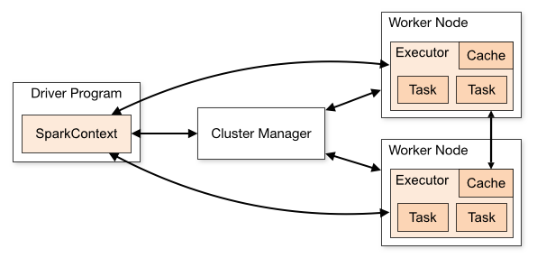
Each program we'll write is a Driver Program. It uses a SparkContext to communicate with the Cluster Manager, which is an abstraction over Hadoop YARN, local mode, standalone (static cluster) mode, Mesos, and EC2.

The Cluster Manager allocates resources. An Executor JVM process is created on each worker node per client application. It manages local resources, such as the cache (see below) and it runs tasks, which are provided by your program in the form of Java jar files or Python scripts.

Because each application has its own executor process per node, applications can't share data through the Spark Context. External storage has to be used (e.g., the file system, a database, a message queue, etc.)

The data caching is one of the key reasons that Spark's performance is considerably better than the performance of MapReduce. Spark stores the data for the job in Resilient, Distributed Datasets (RDDs), where a logical data set is virtualized over the cluster.

The user can specify that data in an RDD should be cached in memory for subsequent reuse. In contrast, MapReduce has no such mechanism, so a complex job requiring a sequence of MapReduce jobs will be penalized by a complete flush to disk of intermediate data, followed by a subsequent reloading into memory by the next job.

RDDs support common data operations, such as map, flatmap, filter, fold/reduce, and groupby. RDDs are resilient in the sense that if a "partition" of data is lost on one node, it can be reconstructed from the original source without having to start the whole job over again.

The architecture of RDDs is described in the research paper Resilient Distributed Datasets: A Fault-Tolerant Abstraction for In-Memory Cluster Computing.

SparkSQL adds the ability to specify schema for RDDs, run SQL queries on them, and even create, delete, and query tables in Hive, the original SQL tool for Hadoop. Recently, support was added for parsing JSON records, inferring their schema, and writing RDDs in JSON format.

Several years ago, the Spark team ported the Hive query engine to Spark, calling it Shark. That port is now deprecated. SparkSQL will replace it once it is feature compatible with Hive. The new query planner is called Catalyst.

This workshop uses Spark 1.1.0.

The following documentation links provide more information about Spark:

• Documentation.
• Scaladocs API.

The Documentation includes a getting-started guide and overviews. You'll find the Scaladocs API useful for the workshop.

Here is a list of the exercises. In subsequent sections, we'll dive into the details for each one. Note that each name ends with a number, indicating the order in which we'll discuss and try them:

• Intro1: The first example is actually run using the interactive spark-shell, as we'll see.
• WordCount2: The Word Count algorithm: Read a corpus of documents, tokenize it into words, and count the occurrences of all the words. A classic, simple algorithm used to learn many Big Data APIs. By default, it uses a file containing the King James Version (KJV) of the Bible. (The data directory has a README that discusses the sources of the data files.)
• WordCount3: An alternative implementation of Word Count that uses a slightly different approach and also uses a library to handle input command-line arguments, demonstrating some idiomatic (but fairly advanced) Scala code.
• Matrix4: Demonstrates using explicit parallelism on a simplistic Matrix application.
• Crawl5a: Simulates a web crawler that builds an index of documents to words, the first step for computing the inverse index used by search engines. The documents "crawled" are sample emails from the Enron email dataset, each of which has been classified already as SPAM or HAM.
• InvertedIndex5b: Using the crawl data, compute the index of words to documents (emails).
• NGrams6: Find all N-word ("NGram") occurrences matching a pattern. In this case, the default is the 4-word phrases in the King James Version of the Bible of the form % love % %, where the % are wild cards. In other words, all 4-grams are found with love as the second word. The % are conveniences; the NGram Phrase can also be a regular expression, e.g., % (hat|lov)ed? % % finds all the phrases with love, loved, hate, and hated.
• Joins7: Spark supports SQL-style joins as shown in this simple example.
• SparkStreaming8: The streaming capability is relatively new and this exercise shows how it works to construct a simple "echo" server. Running it is a little more involved. See below.
• SparkSQL9: Uses the SQL API to run basic queries over structured data, in this case, the same King James Version (KJV) of the Bible used in the previous workshop.
• hadoop/SparkSQLParquet10: Demonstrates writing and reading Parquet-formatted data, namely the data written in the previous example. This example and the next one are in a hadoop subdirectory, because they uses features that require a Hadoop cluster (more details later on).
• hadoop/HiveSQL11: A script that demonstrates interacting with Hive tables (we actually create one) in the Scala REPL!

Let's now work through these exercises...

Intro1.scala

Our first exercise demonstrates the useful Spark Shell, which is a customized version of Scala's REPL (read, eval, print, loop). It allows us to work interactively with our algorithms and data.

Actually, for local mode execution, we won't use the spark-shell command provided by Spark. Instead, we've customized the Activator/SBT console (Scala REPL) to behave in a similar way. For Hadoop execution, we'll use spark-shell.

We'll copy and paste commands from the file Intro1.scala. Click the link to open the file in Activator or open it in your favorite editor/IDE.

The extensive comments in this file and the subsequent files explain the API calls in detail. You can copy and paste the comments, too.

NOTE: while the file extension is .scala, this file is not compiled with the rest of the code, because it works like a script. (The build is configured to not compile this file.)

To run this example on your workstation, you can't use the Activator UI. Quit Activator and use the instructions previously to start it in the shell mode. Once it starts and presents the prompt (Activator-Spark)>, enter the command console. It will compile some code and start the Scala REPL, ending with the prompt scala>. Continue with the instructions below.

In your sandbox or cluster node, change to the root node of the workshop and run the following command:

./scripts/sparkshell.sh

This script calls the actual Spark Shell script, $SPARK_HOME/bin/spark-shell and passes a --jars argument with the jar of the workshop's compiled code. The script also passes any additional arguments you provide to spark-shell. (Try the --help option to see the full list.)

You'll see a lot of log messages, ending with the Scala REPL prompt scala>.

Continue with the instructions below.

Whether you running the REPL in local mode or the spark-shell version in Hadoop, continue with the following steps.

First, there are some commented lines that every Spark program needs, but you don't need to run them now. Both the local Scala REPL configured in the build and the spark-shell variant of the REPL execute these three lines automatically at startup:

// import org.apache.spark.SparkContext
// import org.apache.spark.SparkContext._
// val sc = new SparkContext("local", "Intro (1)")

The SparkContext drives everything else. Why are there two, very similar import statements? The first one imports the SparkContext type so it wouldn't be necessary to use a fully-qualified name in the new SparkContext statement. The second import statement is analogous to a static import in Java, where we make some methods and values visible in the current scope, again without requiring qualification.

When a SparkContext is constructed, there are several constructors that can be used. The one shown takes a string for the "master" and an arbitrary job name. The master must be one of the following:

• local: Start the Spark job standalone and use a single thread to run the job.
• local[k]: Use k threads instead. Should be less than the number of cores.
• mesos://host:port: Connect to a running, Mesos-managed Spark cluster.
• spark://host:port: Connect to a running, standalone Spark cluster.
• yarn-client or yarn-cluster: Connect to a YARN cluster, which we'll use implicitly when we run in Hadoop.

So, actually, the comment shown is only correct for local mode. When you run spark-shell in Hadoop, the actual master argument used is yarn-client.

Next we define a read-only variable input of type RDD by loading the text of the King James Version of the Bible, which has each verse on a line, we then map over the lines converting the text to lower case:

val input = sc.textFile("data/kjvdat.txt").map(line => line.toLowerCase)

The data directory has a README that discusses the files present and where they came from.

Then, we cache the data in memory for faster, repeated retrieval. You shouldn't always do this, as it's wasteful for data that's simply passed through, but when your workflow will repeatedly reread the data, caching provides performance improvements.

input.cache

Next, we filter the input for just those verses that mention "sin" (recall that the text is now lower case). Then count how many were found, convert the RDD to a Scala collection (in the memory for the driver process JVM). Finally, loop through the first twenty lines of the array, printing each one, then we do it again with RDD itself.

val sins = input.filter(line => line.contains("sin"))
val count = sins.count()         // How many sins?
val array = sins.collect()       // Convert the RDD into a collection (array)
array.take(20) foreach println   // Take the first 20, and print them 1/line.
sins.take(20) foreach println    // ... but we don't have to "collect" first;
                                 // we can just use foreach on the RDD.

Note: in Scala, the () in method calls are actually optional for no-argument methods.

Continuing, you can define functions as values. Here we create a separate filter function that we pass as an argument to the filter method. Previously we used an anonymous function. Note that filterFunc is a value that's a function of type String to Boolean.

val filterFunc: String => Boolean =
    (s:String) => s.contains("god") || s.contains("christ")

The following more concise form is equivalent, due to type inference of the argument's type:

val filterFunc: String => Boolean =
    s => s.contains("god") || s.contains("christ")

Now use the filter to find all the sin verses that also mention God or Christ, then count them. Note that this time, we drop the parentheses after "count". Parentheses can be omitted when methods take no arguments.

val sinsPlusGodOrChrist  = sins filter filterFunc
val countPlusGodOrChrist = sinsPlusGodOrChrist.count

A non-script program should gracefully shutdown, but we don't need to do so here. Both our configured console environment for local execution and spark-shell do this for us:

// sc.stop()

If you exit the REPL immediately, this will happen implicitly. Still, it's a good practice to always call stop.

There are comments at the end of this file with suggested exercises to learn the API. All the subsequent examples we'll discuss include suggested exercises, too. Solutions for some of them are provided in the src/main/scala/sparkworkshop/solns directory.

You can exit the Scala REPL now. Type :quit or use ^d (control-d).

If you ran this example locally using the Activator/SBT console, you can exit that application using exit or ^d. Do this if you want to continue using the Activator UI. Restart it as described previously.

WordCount2.scala

The classic, simple Word Count algorithm is easy to understand and it's suitable for parallel computation, so it's a good vehicle when first learning a Big Data API.

In Word Count, you read a corpus of documents, tokenize each one into words, and count the occurrences of all the words globally.

WordCount2.scala uses the KJV Bible text again. (Subsequent exercises will add the ability to specify different input sources using command-line arguments.)

This example does not have a Hadoop version, so we'll only run it locally.

In the Activator UI, select the run panel, then select WordCount2 and click the "Start" button. The messages near the end of the output in the "Logs" panel lists the "output" directory, which is in the local file system, not HDFS.

In the Activator shell or SBT, you can run it one of three ways:

• Enter the run command and select the number corresponding to the WordCount2 program.
• Enter run-main WordCount2
• Enter ex2, a command alias for run-main WordCount2. (The alias is defined in the project's build.sbt file.)

Either way, the output is written to output/kjv-wc2 in the local file system. Use a file browser or another terminal window to view the files in this directory. You'll find an empty _SUCCESS file that marks completion and a part-00000 file that contains the data.

As before, here is the text of the script in sections, with code comments removed:

import com.typesafe.sparkworkshop.util.FileUtil
import org.apache.spark.SparkContext
import org.apache.spark.SparkContext._

We use the Java default package for the compiled exercises, but you would normally include a package ... statement to organize your applications into packages, in the usual Java way.

We import a FileUtil class that we'll use for "housekeeping". Then we use the same two SparkContext imports we discussed previously. This time, they aren't commented; we must specify these imports ourselves in Spark programs.

Even though most of the examples and exercises from now on will be compiled classes, you could still use the Spark Shell to try out most constructs. This is especially useful when experimenting and debugging!

Here is the outline of the rest of the program, demonstrating a pattern we'll use throughout.

object WordCount2 {
  def main(args: Array[String]): Unit = {

    val sc = new SparkContext("local", "Word Count (2)")

    try {
      ...
    } finally {
      sc.stop()      // Stop (shut down) the context.
    }
  }
}

In case the script fails with an exception, putting the SparkContext.stop() inside a finally clause ensures that we'll properly clean up no matter what happens.

The content of the try clause is the following:

val out = "output/kjv-wc2"
FileUtil.rmrf(out)    // Delete old output (if any)

val input = sc.textFile("data/kjvdat.txt").map(line => line.toLowerCase)
input.cache

val wc = input
  .flatMap(line => line.split("""[^\p{IsAlphabetic}]+"""))
  .map(word => (word, 1))
  .reduceByKey((count1, count2) => count1 + count2)

println(s"Writing output to: $out")
wc.saveAsTextFile(out)

Because Spark follows Hadoop conventions that it won't overwrite existing data, we delete any previous output, if any. Of course, you should only do this in production jobs when you know it's okay!

Next we load and cache the data like we did previously, but this time, it's questionable whether caching is useful, since we will make a single pass through the data. I left this statement here just to remind you of this feature.

Now we setup a pipeline of operations to perform the word count.

First the line is split into words using as the separator any run of characters that isn't alphabetic, e.g., digits, whitespace, and punctuation. (Note: using "\\W+" doesn't work well for non-UTF8 character sets!) This also conveniently removes the trailing ~ characters at the end of each line that exist in the file for some reason. input.flatMap(line => line.split(...)) maps over each line, expanding it into a collection of words, yielding a collection of collections of words. The flat part flattens those nested collections into a single, "flat" collection of words.

The next two lines convert the single word "records" into tuples with the word and a count of 1. In Shark, the first field in a tuple will be used as the default key for joins, group-bys, and the reduceByKey we use next.

The reduceByKey step effectively groups all the tuples together with the same word (the key) and then "reduces" the values using the passed in function. In this case, the two counts are added together. Hence, we get two-element records with unique words and their counts.

Finally, we invoke saveAsTextFile to write the final RDD to the output location.

Note that the input and output locations will be relative to the local file system, when running in local mode, and relative to the user's home directory in HDFS (e.g., /user/$USER), when a program runs in Hadoop.

Spark also follows another Hadoop convention for file I/O; the out path is actually interpreted as a directory name. It will contain the same _SUCCESS and part-00000 files discussed previously. In a real cluster with lots of data and lots of concurrent tasks, there would be many part-NNNNN files.

Quiz: If you look at the (unsorted) data, you'll find a lot of entries where the word is a number. (Try "grepping" to find them.) Are there really that many numbers in the bible? If not, where did the numbers come from? Look at the original file for clues.

At the end of each example source file, you'll find exercises you can try. Solutions for some of them are implemented in the solns package. For example, solns/WordCount2GroupBy.scala solves the "group by" exercise described in WordCount2.scala.

WordCount3.scala

This exercise also implements Word Count, but it uses a slightly simpler approach. It also uses a utility library to support command-line arguments, demonstrating some idiomatic (but fairly advanced) Scala code. We won't worry about the details of this utility code, just how to use it. When we set up the SparkContext, we also use Kryo Serialization, which provides better compression and therefore better utilization of memory and network bandwidth.

We'll run this example in both local mode and in Hadoop (YARN).

This version also does some data cleansing to improve the results. The sacred text files included in the data directory, such as kjvdat.txt are actually formatted records of the form:

book|chapter#|verse#|text

That is, pipe-separated fields with the book of the Bible (e.g., Genesis, but abbreviated "Gen"), the chapter and verse numbers, and then the verse text. We just want to count words in the verses, although including the book names wouldn't change the results significantly. (Now you can figure out the answer to the "quiz" in the previous section...)

In the Activator UI, select the run panel, then select WordCount3 and click the "Start" button. The messages near the end of the output in the "Logs" panel lists the "output" directory, which is in the local file system, not HDFS.

In the Activator shell or SBT, you can run it one of three ways, as for WordCount2:

• Enter the run command and select the number corresponding to the WordCount3 program.
• Enter run-main WordCount3
• Enter ex3, a command alias for run-main WordCount3.

You can also run this example in Hadoop. In the Activator UI, select the run panel, then select hadoop.HWordCount3 and click the "Start" button. Now the output directory shown will be in HDFS.

For Activator shell or SBT`, use one of the following:

• Enter the run command and select the number corresponding to the hadoop.HWordCount3 program.
• Enter run-main hadoop.HWordCount3
• Enter hex3, a command alias for run-main hadoop.HWordCount3.

We'll discuss the Hadoop driver in more detail later.

Command line options can be used to override the default settings for input and output locations, among other things. You'll have to use the Activator shell or SBT to use this feature. You can specify arguments after the run, run-main hadoop.HWordCount3, or hex3 commands.

Here is the help message that lists the available options. The "" characters indicate long lines that are wrapped to fit. Enter the commands on a single line without the "". Following Unix conventions, [...] indicates optional arguments, and | indicates alternatives:

run-main WordCount3 [ -h | --help] \
  [-i | --in | --inpath input] \
  [-o | --out | --outpath output] \
  [-m | --master master] \
  [-q | --quiet]

Where the options have the following meanings:

-h | --help     Show help and exit.
-i ... input    Read this input source (default: data/kjvdat.txt).
-o ... output   Write to this output location (default: output/kjvdat-wc3).
-m ... master   local, local[k], yarn-client, etc., as discussed previously.
-q | --quiet    Suppress some informational output.

When running in Hadoop, relative file paths for input our output are interpreted to be relative to /user/$USER in HDFS.

Here is an example that uses the default values for the options:

run-main WordCount3 \
  --inpath data/kjvdat.txt --output output/kjv-wc3 \
  --master local

You can try different variants of local[k] for the master option, but keep k less than the number of cores in your machine or use *.

When you specify an input path for Spark, you can specify bash-style "globs" and even a list of them:

• data/foo: Just the file foo or if it's a directory, all its files, one level deep (unless the program does some extra handling itself).
• data/foo*.txt: All files in data whose names start with foo and end with the .txt extension.
• data/foo*.txt,data2/bar*.dat: A comma-separated list of globs.

Okay, with all the invocation options out of the way, let's walk through the implementation of WordCount3.

WordCount3.scala

We start with import statements:

import com.typesafe.sparkworkshop.util.{CommandLineOptions, FileUtil, TextUtil}
import org.apache.spark.SparkContext
import org.apache.spark.SparkContext._

As before, but with our new CommandLineOptions utilities added.

object WordCount3 {
  def main(args: Array[String]): Unit = {

    val options = CommandLineOptions(
      this.getClass.getSimpleName,
      CommandLineOptions.inputPath("data/kjvdat.txt"),
      CommandLineOptions.outputPath("output/kjv-wc3"),
      CommandLineOptions.master("local"),
      CommandLineOptions.quiet)

    val argz   = options(args.toList)
    val master = argz("master")
    val quiet  = argz("quiet").toBoolean
    val in     = argz("input-path")
    val out    = argz("output-path")

I won't discuss the implementation of CommandLineOptions.scala except to say that it defines some methods that create instances of an Opt type, one for each of the options we discussed above. The single argument given to some of the methods (e.g., CommandLineOptions.inputPath("data/kjvdat.txt")) specifies the default value for that option.

After parsing the options, we extract some of the values we need.

Next, if we're running in local mode, we delete the old output, if any:

    if (master.startsWith("local")) {
      if (!quiet) println(s" **** Deleting old output (if any), $out:")
      FileUtil.rmrf(out)
    }

Note that this logic is only invoked in local mode, because FileUtil only works locally. We also delete old data from HDFS when running in Hadoop, but deletion is handled through a different mechanism, as we'll see shortly.

Now we create a SparkConf to configure the SparkContext with the desired master setting, application name, and the use of Kryo serialization.

    val conf = new SparkConf().setMaster(master).setAppName("Word Count (3)")
    conf.set("spark.serializer", "org.apache.spark.serializer.KryoSerializer")
    // conf.registerKryoClasses(Array(classOf[MyCustomClass]))
    val sc = new SparkContext(master, "Word Count (3)")

Note the commented line. For best use of Kryo, you should "register" the classes you'll be serializing. However, Kryo already "knows" about common types, such as String, which is what we're using here, so we don't need this statement.

Now we process the input as before, with one change...

    try {
      val input = sc.textFile(argz("input-path"))
        .map(line => TextUtil.toText(line)) // also converts to lower case

It starts out much like WordCount2, but it uses a helper method TextUtil.toText to split each line from the religious texts into fields, where the lines are of the form: book|chapter#|verse#|text. The | is the field delimiter. However, if other inputs are used, their text is returned unmodified. As before, the input reference is an RDD. NOte that I omitted a subsequent call to input.cache as in WordCount2, because we are making a single pass through the data.

      val wc2 = input
        .flatMap(line => line.split("""[^\p{IsAlphabetic}]+"""))
        .countByValue()  // Returns a Map[T, Long]

Take input and split on non-alphabetic sequences of character as we did in WordCount2, but rather than map to (word, 1) tuples and use reduceByKey, we simply treat the words as values and call countByValue to count the unique occurrences. Hence, this is a simpler and more efficient approach.

      val wc2b = wc2a.map(key_value => s"${key_value._1},${key_value._2}").toSeq
      val wc2 = sc.makeRDD(wc2b, 1)

      if (!quiet) println(s"Writing output to: $out")
      wc2.saveAsTextFile(out)

    } finally {
      sc.stop()
    }
  }
}

The result of countByValue is a Scala Map, not an RDD, so we format the key-value pairs into a sequence of strings in comma-separated value (CSV) format. The we convert this sequence back to an RDD with makeRDD. Finally, we save to the file system as text.

In a previous section, we described how to run WordCount3 either locally or in Hadoop. Let's discuss the Hadoop details now.

Recall from the setup instructions that the data must already be in HDFS. The location /user/$USER/data is assumed. If you used a different location, always specify the --input argument when you run the examples.

The driver program, hadoop.HWordCound3, is used to run WordCount3 in Hadoop. It is also available in the Activator UI Run panel and the shell/SBT run command. Try it now.

The output is more verbose and the execution time is longer, due to Hadoop's overhead. The end of the output shows a URL for the Hue UI that's also part of the Sandbox. Open your browser to that URL to look at the data. The content will be very similar to the output of the previous, local run, but it will be formatted differently and the word-count pairs will be in a different (random) order.

Using the Activator shell or SBT, you can also use run-main hadoop.HWordCount3 or the alias hex3.

For convenient, there is also a bash shell script for this example in the scripts directory, scripts.wordcount3.sh:

#!/bin/bash

output=output/kjv-wc3
dir=$(dirname $0)
$dir/hadoop.sh --class WordCount3 --output "$output" "$@"

It calls a scripts.hadoop.sh script in the same directory, which deletes the old output from HDFS, if any, and calls Spark's $SPARK_HOME/bin/spark-submit to submit the job to YARN. One of the arguments it passes to spark-submit is the jar file containing all the project code. This jar file is built automatically anytime you invoke the Activator run command.

The other examples also have corresponding scripts and driver programs.

Let's return to hadoop.HWordCound3, which is quite small:

package hadoop
import com.typesafe.sparkworkshop.util.Hadoop

object HWordCount3 {
  def main(args: Array[String]): Unit = {
    Hadoop("WordCount3", "output/kjv-wc3", args)
  }
}

It accepts the same options as WordCount3, although the --master option defaults to yarn-client this time.

It delegates to a helper class com.typesafe.sparkworkshop.util.Hadoop to do the work. It passes as arguments the class name and the output location. The second argument is a hack: the default output path must be specified here, even though the same default value is also encoded in the application. This is because we eventually pass the value to the hadoop.sh script, which uses it to delete an old output directory, if any.

Here is the Hadoop helper class:

package com.typesafe.sparkworkshop.util
import scala.sys.process._

object Hadoop {
  def apply(className: String, defaultOutpath: String, args: Array[String]): Unit = {
    val user = sys.env.get("USER") match {
      case Some(user) => user
      case None =>
        println("ERROR: USER environment variable isn't defined. Using root!")
        "root"
    }

    // Did the user specify an output path? Use it instead.
    val predicate = (arg: String) => arg.startsWith("-o") || arg.startsWith("--o")
    val args2 = args.dropWhile(arg => !predicate(arg))
    val outpath = if (args2.size == 0) s"/user/$user/$defaultOutpath"
      else if (args2(1).startsWith("/")) args2(1)
      else s"/user/$user/${args(2)}"

    // We don't need to remove the output argument. A redundant occurrence
    // is harmless.
    val argsString = args.mkString(" ")
    val exitCode = s"scripts/hadoop.sh --class $className --out $outpath $argsString".!
    if (exitCode != 0) sys.exit(exitCode)
  }
}

It tries to determine the user name and whether or not the user explicitly specified an output argument, which should override the hard-coded value.

Finally, it invokes the scripts.hadoop.sh bash script we mentioned above, so that we go thorugh Spark's spark-submit script for submitting to the Hadoop YARN cluster.

WordCount3.scala

Don't forget the try the exercises at the end of the source file.

For Hadoop execution, you'll need to edit the source code on cluster or edge node or the sandbox. One way is to simply use an editor on the node, i.e., vi or emacs to edit the code. Another approach is to use the secure copy command, scp, to copy edited sources to and from your workstation.

For sandboxes, the best approach is to share this workshop's root directory between your workstation and the VM Linux instance. This will allow you to edit the code in your workstation environment with the changes immediately available in the VM. See the documentation for your VM runner for details on sharing folders.

For example, in VMWare, the Sharing panel lets you specify workstation directories to share. In the Linux VM, run the following commands as root to mount all shared directories under /home/shares (or use a different location):

mkdir -p /home/shares
mount -t vmhgfs .host:/ /home/shares

Now any shared workstation folders will appear under /home/shares.

Matrix4.scala

An early use for Spark was implementing Machine Learning algorithms. Spark's MLlib of algorithms contains classes for vectors and matrices, which are important for many ML algorithms. This exercise uses a simpler representation of matrices to explore another topic; explicit parallelism.

The sample data is generated internally; there is no input that is read. The output is written to the file system as before.

Here is the run-main command with optional arguments:

run-main Matrix4 [ -h | --help] \
  [-d | --dims NxM] \
  [-o | --out | --outpath output] \
  [-m | --master master] \
  [-q | --quiet]

The one new optin is for specifying the dimensions, where the string NxM is parsed to mean N rows and M columns. The default is 5x10.

Like for WordCount3, there is also a ex4 short cut for run-main Matrix4 and you can run with the default arguments using the Activator Run panel.

For Hadoop, select and run hadoop.HMatrix4 in the UI, use run-main hadoop.HMatrix4 or hex4 in the Activator shell, and there is a bash script scripts/matrix4.sh.

We won't cover all the code from now on; we'll skip the familiar stuff:

import com.typesafe.sparkworkshop.util.Matrix
...

object Matrix4 {

  case class Dimensions(m: Int, n: Int)

  def main(args: Array[String]): Unit = {

    val options = CommandLineOptions(...)
    val argz   = options(args.toList)
    ...

    val dimsRE = """(\d+)\s*x\s*(\d+)""".r
    val dimensions = argz("dims") match {
      case dimsRE(m, n) => Dimensions(m.toInt, n.toInt)
      case s =>
        println("""Expected matrix dimensions 'NxM', but got this: $s""")
        sys.exit(1)
    }

Dimensions is a convenience class for capturing the default or user-specified matrix dimensions. We parse the argument string to extract N and M, then construct a Dimension instance.

    val sc = new SparkContext("local", "Matrix (4)")

    try {
      // Set up a mxn matrix of numbers.
      val matrix = Matrix(dimensions.m, dimensions.n)

      // Average rows of the matrix in parallel:
      val sums_avgs = sc.parallelize(1 to dimensions.m).map { i =>
        // Matrix indices count from 0.
        // "_ + _" is the same as "(count1, count2) => count1 + count2".
        val sum = matrix(i-1) reduce (_ + _)
        (sum, sum/dimensions.n)
      }.collect    // convert to an array

The core of this example is the use of SparkContext.parallelize to process each row in parallel (subject to the available cores on the machine or cluster, of course). In this case, we sum the values in each row and compute the average.

The argument to parallelize is a sequence of "things" where each one will be passed to one of the operations. Here, we just use the literal syntax to construct a sequence of integers from 1 to the number of rows. When the anonymous function is called, one of those row numbers will get assigned to i. We then grab the i-1 row (because of zero indexing) and use the reduce method to sum the column elements. A final tuple with the sum and the average is returned.

      // Make a new sequence of strings with the formatted output, then we'll
      // dump to the output location.
      val outputLines = Vector(          // Scala's Vector, not MLlib's version!
        s"${dimensions.m}x${dimensions.n} Matrix:") ++ sums_avgs.zipWithIndex.map {
        case ((sum, avg), index) =>
          f"Row #${index}%2d: Sum = ${sum}%4d, Avg = ${avg}%3d"
      }
      val output = sc.makeRDD(outputLines)  // convert back to an RDD
      if (!quiet) println(s"Writing output to: $out")
      output.saveAsTextFile(out)
    } finally { ... }
  }
}

The output is formatted as a sequence of strings and converted back to an RDD for output. The expression sums_avgs.zipWithIndex creates a tuple with each sums_avgs value and it's index into the collection. We use that to add the row index to the output.

Try the simple exercises at the end of the source file.

Crawl5a.scala

The fifth example is in two-parts. The first part simulates a web crawler that builds an index of documents to words, the first step for computing the inverse index used by search engines, from words to documents. The documents "crawled" are sample emails from the Enron email dataset, each of which has been previously classified already as SPAM or HAM.

Crawl5a supports the same command-line options as WordCount3:

run-main Crawl5a [ -h | --help] \
  [-i | --in | --inpath input] \
  [-o | --out | --outpath output] \
  [-m | --master master] \
  [-q | --quiet]

As before, there is also a ex5a short cut for run-main Crawl5a and you can run with the default arguments using the Activator Run panel.

Crawl5a uses a convenient SparkContext method wholeTextFiles, which is given a directory "glob". The default we use is data/enron-spam-ham/*, which expands to data/enron-spam-ham/ham100 and data/enron-spam-ham/spam100. This method returns records of the form (file_name, file_contents), where the file_name is the absolute path to a file found in one of the directories, and file_contents contains its contents, including nested linefeeds. To make it easier to run unit tests, Crawl5a strips off the leading path elements in the file name (not normally recommended) and it removes the embedded linefeeds, so that each final record is on a single line.

Here is an example line from the output :

(0038.2001-08-05.SA_and_HP.spam.txt,  Subject: free foreign currency newsletter ...)

The next step has to parse this data to generate the inverted index.

Note: There is also an older Crawl5aLocal included but no longer used. It works similarly, but for local file systems only.

InvertedIndex5b.scala

Using the crawl data just generated, compute the index of words to documents (emails). This is a simple approach to building a data set that could be used by a search engine. Each record will have two fields, a word and a list of tuples of documents where the word occurs and a count of the occurrences in the document.

InvertedIndex5b supports the usual command-line options:

run-main InvertedIndex5b [ -h | --help] \
  [-i | --in | --inpath input] \
  [-o | --out | --outpath output] \
  [-m | --master master] \
  [-q | --quiet]

For Hadoop, select and run hadoop.HInvertedIndex5b in the UI, use run-main hadoop.HInvertedIndex5b or hex5b in the Activator shell. There is also a bash script scripts/invertedindex5b.sh.

The code outside the try clause follows the usual pattern, so we'll focus on the contents of the try clause:

try {
  val lineRE = """^\s*\(([^,]+),(.*)\)\s*$""".r
  val input = sc.textFile(argz("input-path")) map {
    case lineRE(name, text) => (name.trim, text.toLowerCase)
    case badLine =>
      Console.err.println("Unexpected line: $badLine")
      ("", "")
  }

We load the "crawl" data, where each line was written by Crawl5a with the following format: (document_id, text) (including the parentheses). Hence, we use a regular expression with "capture groups" to extract the document_id and text.

Note the function passed to map. It has the form:

{
  case lineRE(name, text) => ...
  case line => ...
}

There is now explicit argument list like we've used before. This syntax is the literal syntax for a partial function, a mathematical concept for a function that is not defined at all of its inputs. It is implemented with Scala's PartialFunction type.

We have two case match clauses, one for when the regular expression successfully matches and returns the capture groups into variables name and text and the second which will match everything else, assigning the line to the variable badLine. (In fact, this catch-all clause makes the function total, not partial.) The function must return a two-element tuple, so the catch clause simply returns ("","").

Note that the specified or default input-path is a directory with Hadoop-style content, as discussed previously. Spark knows to ignore the "hidden" files.

The embedded comments in the rest of the code explains each step:

if (!quiet)  println(s"Writing output to: $out")

// Split on non-alphabetic sequences of character as before.
// Rather than map to "(word, 1)" tuples, we treat the words by values
// and count the unique occurrences.
input
  .flatMap {
    // all lines are two-tuples; extract the path and text into variables
    // named "path" and "text".
    case (path, text) =>
      // If we don't trim leading whitespace, the regex split creates
      // an undesired leading "" word!
      text.trim.split("""[^\p{IsAlphabetic}]+""") map (word => (word, path))
  }
  .map {
    // We're going to use the (word, path) tuple as a key for counting
    // all of them that are the same. So, create a new tuple with the
    // pair as the key and an initial count of "1".
    case (word, path) => ((word, path), 1)
  }
  .reduceByKey{    // Count the equal (word, path) pairs, as before
    (count1, count2) => count1 + count2
  }
  .map {           // Rearrange the tuples; word is now the key we want.
    case ((word, path), n) => (word, (path, n))
  }
  .groupByKey      // There is a also a more general groupBy
  // reformat the output; make a string of each group,
  // a sequence, "(path1, n1) (path2, n2), (path3, n3)..."
  .mapValues(iterator => iterator.mkString(", "))
  // mapValues is like the following map, but more efficient, as we skip
  // pattern matching on the key ("word"), etc.
  // .map {
  //   case (word, seq) => (word, seq.mkString(", "))
  // }
  .saveAsTextFile(out)
} finally { ... }

Each output record has the following form: (word, (doc1, n1), (doc2, n2), ...). For example, the word "ability" appears twice in one email and once in another (both SPAM):

(ability,(0018.2003-12-18.GP.spam.txt,2), (0020.2001-07-28.SA_and_HP.spam.txt,1))

It's worth studying this sequence of transformations to understand how it works. Many problems can be solves with these techniques. You might try reading a smaller input file (say the first 5 lines of the crawl output), then hack on the script to dump the RDD after each step.

A few useful RDD methods for exploration include RDD.sample or RDD.take, to select a subset of elements. Use RDD.saveAsTextFile to write to a file or use RDD.collect to convert the RDD data into a "regular" Scala collection (don't use for massive data sets!).

NGrams6.scala

In Natural Language Processing, one goal is to determine the sentiment or meaning of text. One technique that helps do this is to locate the most frequently-occurring, N-word phrases, or NGrams. Longer NGrams can convey more meaning, but they occur less frequently so all of them appear important. Shorter NGrams have better statistics, but each one conveys less meaning. In most cases, N = 3-5 appears to provide the best balance.

This exercise finds all NGrams matching a user-specified pattern. The default is the 4-word phrases the form % love % %, where the % are wild cards. In other words, all 4-grams are found with love as the second word. The % are conveniences; the user can also specify an NGram Phrase that is a regular expression or a mixture, e.g., % (hat|lov)ed? % % finds all the phrases with love, loved, hate, or hated as the second word.

NGrams6 supports the same command-line options as WordCount3, plus two new options:

run-main NGrams6 [ -h | --help] \
  [-i | --in | --inpath input] \
  [-o | --out | --outpath output] \
  [-m | --master master] \
  [-c | --count N] \
  [-n | --ngrams string] \
  [-q | --quiet]

Where

-c | --count N        List the N most frequently occurring NGrams (default: 100)
-n | --ngrams string  Match string (default "% love % %"). Quote the string!

For Hadoop, select and run hadoop.HNGrams6 in the UI, use run-main hadoop.HNGrams6 or hex6 in the Activator shell. There is also a bash script scripts/ngrams6.sh.

I'm in yür codez:

...
val ngramsStr = argz("ngrams").toLowerCase
val ngramsRE = ngramsStr.replaceAll("%", """\\w+""").replaceAll("\\s+", """\\s+""").r
val n = argz("count").toInt

From the two new options, we get the ngrams string. Each % is replaced by a regex to match a word and whitespace is replaced by a general regex for whitespace.

try {
  object CountOrdering extends Ordering[(String,Int)] {
    def compare(a:(String,Int), b:(String,Int)) =
      -(a._2 compare b._2)  // - so that it sorts descending
  }

  val ngramz = sc.textFile(argz("input-path"))
    .flatMap { line =>
        val text = TextUtil.toText(line) // also converts to lower case
        ngramsRE.findAllMatchIn(text).map(_.toString)
    }
    .map(ngram => (ngram, 1))
    .reduceByKey((count1, count2) => count1 + count2)
    .takeOrdered(n)(CountOrdering)

We need an implementation of Ordering to sort our found NGrams descending by count.

We read the data as before, but note that because of our line orientation, we won't find NGrams that cross line boundaries! This doesn't matter for our sacred text files, since it wouldn't make sense to find NGrams across verse boundaries, but a more flexible implementation should account for this. Note that we also look at just the verse text, as in WordCount3.

The map and reduceByKey calls are just like we used previously for WordCount2, but now we're counting found NGrams. The takeOrdered call combines sorting with taking the top n found. This is more efficient than separate sort, then take operations. As a rule, when you see a method that does two things like this, it's usually there for efficiency reasons!

The rest of the code formats the results and converts them to a new RDD for output:

  // Format the output as a sequence of strings, then convert back to
  // an RDD for output.
  val outputLines = Vector(
    s"Found ${ngramz.size} ngrams:") ++ ngramz.map {
    case (ngram, count) => "%30s\t%d".format(ngram, count)
  }

  val output = sc.makeRDD(outputLines)  // convert back to an RDD
  if (!quiet) println(s"Writing output to: $out")
  output.saveAsTextFile(out)
} finally { ... }

Joins7.scala

Joins are a familiar concept in databases and Spark supports them, too. Joins at very large scale can be quite expensive, although a number of optimizations have been developed, some of which require programmer intervention to use. We won't discuss the details here, but it's worth reading how joins are implemented in various Big Data systems, such as this discussion for Hive joins and the Joins section of Hadoop: The Definitive Guide.

Here, we will join the KJV Bible data with a small "table" that maps the book abbreviations to the full names, e.g., Gen to Genesis.

Joins7 supports the following command-line options:

run-main Joins7 [ -h | --help] \
  [-i | --in | --inpath input] \
  [-o | --out | --outpath output] \
  [-m | --master master] \
  [-a | --abbreviations path] \
  [-q | --quiet]

Where the --abbreviations is the path to the file with book abbreviations to book names. It defaults to data/abbrevs-to-names.tsv. Note that the format is tab-separated values, which the script must handle correctly.

For Hadoop, select and run hadoop.HJoins7 in the UI, use run-main hadoop.HJoins7 or hex7 in the Activator shell. There is also a bash script scripts/joins7.sh.

Here r yür codez:

...
try {
  val input = sc.textFile(argz("input-path"))
    .map { line =>
      val ary = line.split("\\s*\\|\\s*")
      (ary(0), (ary(1), ary(2), ary(3)))
    }

The input sacred text (default: data/kjvdat.txt) is assumed to have the format book|chapter#|verse#|text. We split on the delimiter and output a two-element tuple with the book abbreviation as the first element and a nested tuple with the other three elements. For joins, Spark wants a (key,value) tuple, which is why we use the nested tuple.

The abbreviations file is handled similarly, but the delimiter is a tab:

val abbrevs = sc.textFile(argz("abbreviations"))
  .map{ line =>
    val ary = line.split("\\s+", 2)
    (ary(0), ary(1).trim)  // I've noticed trailing whitespace...
  }

Note the second argument to split. Just in case a full book name has a nested tab, we explicitly only want to split on the first tab found, yielding two strings.

// Cache both RDDs in memory for fast, repeated access.
input.cache
abbrevs.cache

// Join on the key, the first field in the tuples; the book abbreviation.

val verses = input.join(abbrevs)

if (input.count != verses.count) {
  println(s"input count != verses count (${input.count} != ${verses.count})")
}

We perform an inner join on the keys of each RDD and add a sanity check for the output. Since this is an inner join, the sanity check catches the case where an abbreviation wasn't found and the corresponding verses were dropped!

The schema of verses is this: (key, (value1, value2)), where value1 is (chapter, verse, text) from the KJV input and value2 is the full book name, the second "field" from the abbreviations file. We now flatten the records to the final desired form, fullBookName|chapter|verse|text:

val verses2 = verses map {
  // Drop the key - the abbreviated book name
  case (_, ((chapter, verse, text), fullBookName)) =>
    (fullBookName, chapter, verse, text)
}

Lastly, we write the output:

  if (!quiet) println(s"Writing output to: $out")
  verses2.saveAsTextFile(out)
} finally { ... }

The join method we used is implemented by spark.rdd.PairRDDFunctions, with many other methods for computing "co-groups", outer joins, etc.

You can verify that the output file looks like the input KJV file with the book abbreviations replaced with the full names. However, as currently written, the books are not retained in the correct order! (See the exercises in the source file.)

SparkStreaming8.scala

The streaming capability is relatively new and this exercise uses it to construct a simple "word count" server. The example has two running configurations, reflecting the basic input sources supported by Spark Streaming.

In the first configuration, which is also the default behavior for this example, new data is read from files that appear in a directory. This approach supports a workflow where new files are written to a landing directory and Spark Streaming is used to detect them, ingest them, and process the data.

Note that Spark Streaming does not use the _SUCCESS marker file we mentioned earlier, in part because that mechanism can only be used once all files are written to the directory. Hence, only use this ingestion mechanism with files that "appear instantly" in the directory, i.e., through renaming from another location in the file system.

The second basic configuration reads data from a socket. Spark Streaming also comes with connectors for other data sources, such as Apache Kafka and Twitter streams. We don't explore those here.

SparkStreaming8 uses directory watching by default. A temporary directory is created and a second process writes the KJV Bible file to a temporary file in the directory every few seconds. Hence, the data will be same in every file, but stream processing with read each new file on each iteration. SparkStreaming8 does Word Count on the data.

The socket option works similarly. By default, the same KJV file is written over and over again to a socket.

In either configuration, we need a second process or dedicated thread to either write new files to the watch directory or over the socket. To support this, SparkStreaming8Main.scala is the actual driver program we'll run. It uses two helper classes, com.typesafe.sparkworkshop.util.streaming.DataDirectoryServer.scala and com.typesafe.sparkworkshop.util.streaming.DataSocketServer.scala, respectively. It runs their logic in a separate thread, although each can also be run as a separate executable. Command line options specify which one to use and it defaults to DataSocketServer.

So, let's run this configuration first. In Activator or SBT, run SparkStreaming8Main (not SparkStreaming8MainSocket) as we've done for the other exercises. For the Activator shell or SBT prompt, the corresponding alias is now ex8directory, instead of ex8.

This driver uses DataSocketServer to periodically write copies of the KJV Bible text file to a temporary directory tmp/streaming-input, while it also runs SparkStreaming8 with options to watch this directory. Execution is terminated after 30 seconds, because otherwise the app will run forever!

If you watch the console output, you'll see messages like this:

-------------------------------------------
Time: 1413724627000 ms
-------------------------------------------
(Oshea,2)
(winefat,2)
(cleaveth,13)
(bone,19)
(House,1)
(Shimri,3)
(pygarg,1)
(nobleman,3)
(honeycomb,9)
(manifestly,1)
...

The time stamp will increment by 2000 ms each time, because we're running with 2-second batch intervals. This particular output comes from the print method in the program (discussed below), which is a useful debug tool for seeing the first 10 or so values in the current batch RDD.

At the same time, you'll see new directories appear in output, one per batch. They are named like output/wc-streaming-1413724628000.out, again with a timestamp appended to our default output argument output/wc-streaming. Each of these will contain the usual _SUCCESS and part-0000N files, one for each core that the job can get!

Now let's run with socket input. In Activator or SBT, run SparkStreaming8MainSocket. For the Activator shell or SBT prompt, the corresponding alias is now ex8socket. In either case, this is equivalent to passing the extra option --socket localhost:9900 to SparkStreaming8Main, telling it spawn a thread running an instance of DataSocketServer to write data to a socket at this address. SparkStreaming8 will read this socket. the same data file (KJV text by default) will be written over and over again to this socket.

The console output and the directory output should be very similar to the output of the previous run.

SparkStreaming8 supports the following command-line options:

run-main SparkStreaming8 [ -h | --help] \
  [-i | --in | --inpath input] \
  [-s | --socket server:port] \
  [--term | --terminate N] \
  [-q | --quiet]

Where the default is --inpath tmp/wc-streaming. This is the directory that will be watched for data, which DataDirectoryserver will populate. However, the --inpath argument is ignored if the --socket argument is given.

By default, 30 seconds is used for the terminate option, after which time it exits. Pass 0 for no termination.

Note that there's no argument for the data file. That's an extra option supported by SparkStreaming8Main (SparkStreaming8 is agnostic to the source!):

  -d | --data  file

The default is data/kjvdat.txt.

To run the same logic in Hadoop, there is hadoop.HSparkStreaming8 driver. Similarly to SparkStreaming8Main, it starts the DataSocketSever process locally (outside of Hadoop), then submits SparkStreaming8 to your Hadoop environment. There is also a script driver, scripts/sparkstreaming8.sh.

Note that the Hadoop implementation of this example doesn't support watching for new files in a directory. That's not a Spark Streaming limitation.

Spark Streaming uses a clever hack; it runs more or less the same Spark API (or code that at least looks conceptually the same) on deltas of data, say all the events received within one-second intervals (which is what we used here). Deltas of one second to several minutes are most common. Each delta of events is stored in its own RDD encapsulated in a DStream ("Discretized Stream").

You can also define a moving window over one or more batches, for example if you want to compute running statistics.

A StreamingContext is used to wrap the normal SparkContext, too.

Here are the key parts of the code for SparkStreaming8.scala:

...
case class EndOfStreamListener(sc: StreamingContext) extends StreamingListener {
  override def onReceiverError(error: StreamingListenerReceiverError):Unit = {
    out.println(s"Receiver Error: $error. Stopping...")
    sc.stop()
  }
  override def onReceiverStopped(stopped: StreamingListenerReceiverStopped):Unit = {
    out.println(s"Receiver Stopped: $stopped. Stopping...")
    sc.stop()
  }
}

The EndOfStreamListener will be used to detect when a socket connection drops. It will start the exit process. Note that it is not triggered when the end of file is reached while reading directories of files. In this case, we have to rely on the 5-second timeout to quit.

...
val conf = new SparkConf()
         .setMaster("local[*]")
         .setAppName("Spark Streaming (8)")
         .set("spark.cleaner.ttl", "60")
         .set("spark.files.overwrite", "true")
         // If you need more memory:
         // .set("spark.executor.memory", "1g")
val sc  = new SparkContext(conf)

Construct the SparkContext a different way, by first defining a SparkConf (configuration) object. First, it is necessary to use at least 2 cores when running locally to avoid a problem discussed here. We use * to let it use as many cores as it can, setMaster("local[*]")

Spark Streaming requires the TTL to be set, spark.cleaner.ttl, which defaults to infinite. This specifies the duration in seconds for how long Spark should remember any metadata, such as the stages and tasks generated, etc. Periodic clean-ups are necessary for long-running streaming jobs. Note that an RDD that persists in memory for more than this duration will be cleared as well. See Configuration for more details.

With the SparkContext, we create a StreamingContext, where we also specify the time interval, 2 seconds. The best choice will depend on the data rate, how soon the events need processing, etc. Then, we add a listener for socket drops:

val ssc = new StreamingContext(sc, Seconds(2))
ssc.addStreamingListener(EndOfStreamListener(ssc))

If a socket connection wasn't specified, then use the input-path to read from one or more files (the default case). Otherwise use a socket. An InputDStream is returned in either case as lines. The two methods useDirectory and useSocket are listed below.

try {
  val lines =
    if (argz("socket") == "") useDirectory(ssc, argz("input-path"))
    else useSocket(ssc, argz("socket"))

The lines value is a DStream (Discretized Stream) that encapsulates the logic for listening to a socket or watching for new files in a directory. At each batch interval (2 seconds in our case), an RDD will be generated to hold the events received in that interval. For low data rates, an RDD could be empty.

Now we implement an incremental word count:

  val words = lines.flatMap(line => line.split("""[^\p{IsAlphabetic}]+"""))

  val pairs = words.map(word => (word, 1))
  val wordCounts = pairs.transform(rdd => rdd.reduceByKey(_ + _))

  wordCounts.print()  // print a few counts...

  // Generates a new, timestamped directory for each batch interval.
  if (!quiet) println(s"Writing output to: $out")
  wordCounts.saveAsTextFiles(out, "out")

  ssc.start()
  if (term > 0) ssc.awaitTermination(term * 1000)
  else ssc.awaitTermination()

} finally {
  // Having the ssc.stop here is only needed when we use the timeout.
  out.println("+++++++++++++ Stopping! +++++++++++++")
  ssc.stop()
}

This works much like our previous word count logic, except for the use of transform, a DStream method for transforming the RDDs into new RDDs. In this case, we are performing "mini-word counts", within each RDD, but not across the whole DStream.

The DStream also provides the ability to do window operations, e.g., a moving average over the last N intervals.

Lastly, we wait for termination. The term value is the number of seconds to run before terminating. The default value is 30 seconds, but the user can specify a value of 0 to mean no termination.

The code ends with useSocket and useDirectory:

  private def useSocket(sc: StreamingContext, serverPort: String): DStream[String] = {
    try {
      // Pattern match to extract the 0th, 1st array elements after the split.
      val Array(server, port) = serverPort.split(":")
      out.println(s"Connecting to $server:$port...")
      sc.socketTextStream(server, port.toInt)
    } catch {
      case th: Throwable =>
        sc.stop()
        throw new RuntimeException(
          s"Failed to initialize host:port socket with host:port string '$serverPort':",
          th)
    }
  }

  // Hadoop text file compatible.
  private def useDirectory(sc: StreamingContext, dirName: String): DStream[String] = {
    out.println(s"Reading 'events' from directory $dirName")
    sc.textFileStream(dirName)
  }
}

See also SparkStreaming8Main.scala, the main driver, and the helper classes for feeding data to the example, DataDirectoryServer.scala and DataSocketServer.scala.

This is just the tip of the iceberg for Streaming. See the Streaming Programming Guide for more information.

SparkSQL9.scala

The last set of examples and exercises explores the new SparkSQL API, which extends RDDs with a "schema" for records, defined using Scala case classes, and allows you to embed queries using a subset of SQL in strings, as a supplement to the regular manipulation methods on the RDD type; use the best tool for the job in the same application! There is also a builder DSL for constructing these queries, rather than using SQL strings.

Furthermore, SparkSQL can read and write the new Parquet format that's becoming popular in Hadoop environments. SparkSQL also supports parsing JSON-formatted records, with inferred schemas, and writing RDDs in JSON.

Finally, SparkSQL embeds access to a Hive metastore, so you can create and delete tables, and run queries against them using Hive's query language, HiveQL.

This example treats the KJV text we've been using as a table with a schema. It runs several queries on the data.

There is a SparkSQL9.scala program that you can run as before using Activator or SBT. However, SQL queries are more interesting when used interactively. So, there's also a "script" version called SparkSQL9-script.scala, which we'll look at instead. (There are minor differences in how output is handled.)

The codez:

import com.typesafe.sparkworkshop.util.Verse
import org.apache.spark.sql.SQLContext
import org.apache.spark.rdd.RDD

The helper class Verse will be used to define the schema for Bible verses. Note the new imports.

Next, define a convenience function for taking the first n records of an RDD (n defaults to 100) and printing each one to the console:

def dump(rdd: RDD[_], n: Int = 100) =
  rdd.take(n).foreach(println) // Take the first n lines, then print them.

Now create a SQLContext that wraps the SparkContext, just like the StreamingContext did. We don't show this here, but in fact you can mix SparkSQL and Spark Streaming in the same program.

val sc = new SparkContext(argz("master"), "Spark SQL (9)")
val sqlc = new SQLContext(sc)
import sqlc._

The import statement brings SQL-specific functions and values in scope. (Scala allows importing members of objects, while Java only allows importing static members of classes.)

Next we use a regex to parse the input verses and extract the book abbreviation, chapter number, verse number, and text. The fields are separated by "|", and also removes the trailing "~" unique to this file. Then it invokes flatMap over the file lines (each considered a record) to extract each "good" lines and convert them into a Verse instances. Verse is defined in the util package. If a line is bad, a log message is written and an empty sequence is returned. Using flatMap and sequences means we'll effectively remove the bad lines.

We use flatMap over the results so that lines that fail to parse are essentially put into empty lists that will be ignored.

// Regex to match the fields separated by "|".
// Also strips the trailing "~" in the KJV file.
val lineRE = """^\s*([^|]+)\s*\|\s*([\d]+)\s*\|\s*([\d]+)\s*\|\s*(.*)~?\s*$""".r
// Use flatMap to effectively remove bad lines.
val verses = sc.textFile(argz("input-path")) flatMap {
  case lineRE(book, chapter, verse, text) =>
    Seq(Verse(book, chapter.toInt, verse.toInt, text))
  case line =>
    Console.err.println("Unexpected line: $line")
    Seq.empty[Verse]  // Will be eliminated by flattening.
}

Register the RDD as a temporary "table", so we can write SQL queries against it. As the name implies, this "table" only exists for the life of the process. Then we write queries and save the results back to the file system.

verses.registerTempTable("kjv_bible")
verses.cache()
dump(verses)  // print the 1st 100 lines

val godVerses = sql("SELECT * FROM kjv_bible WHERE text LIKE '%God%'")
println("Number of verses that mention God: "+godVerses.count())
dump(godVerses)  // print the 1st 100 lines

val counts = sql("SELECT book, COUNT(*) FROM kjv_bible GROUP BY book")
  // Collect all partitions into 1 partition. Otherwise, there are 100s
  // output from the last query!
  .coalesce(1)
dump(counts)  // print the 1st 100 lines

Note that the SQL dialect currently supported by the sql method is a subset of HiveSQL. For example, it doesn't permit column aliasing, e.g., COUNT(*) AS count. Nor does it appear to support WHERE clauses in some situations.

So, how do we use this script? To run it in Hadoop, you can run the script using the following helper script in the scripts directory:

scripts/sparkshell.sh src/main/scala/sparkworkshop/SparkSQL9-script.scala

Alternatively, start the interactive shell and then copy and past the statements one at a time to see what they do. I recommend this approach for the first time:

scripts/sparkshell.sh

Th sparkshell.sh script does some set up, but essentially its equivalent to the following:

$SPARK_HOME/bin/spark-shell \
  --jars target/scala-2.10/activator-spark_2.10-3.4.0.jar [arguments]

The jar file contains all the project's build artifacts (but not the dependencies).

To run this script locally, use the Activator shell's console command. Assuming you're at the shell's prompt >, use the following commands to enter the Scala interpreter ("REPL") and then load and run the whole file.

(Activator-Spark)> console
scala> :load src/main/scala/sparkworkshop/SparkSQL9-script.scala
...
scala> :quit
(Activator-Spark)> exit

To enter the statements using copy and paste, just paste them at the scala> prompt instead of loading the file.

SparkSQLParquet10.scala

This script demonstrates the methods for reading and writing files in the Parquet format. It reads in the same data as in the previous example, writes it to new files in Parquet format, then reads it back in and runs queries on it.

NOTE: Running this script requires a Hadoop installation, therefore it won't work in local mode, i.e., the Activator shell console. This is why it is in a hadoop sub-package.

The key SchemaRDD methods are SchemaRDD.saveAsParquetFile(outpath) and SqlContext.parquetFile(inpath). The rest of the details are very similar to the previous exercise.

See the script for more details. Run it in Hadoop using the same techniques as for SparkSQL9-script.scala.

HiveSQL11.scala

The previous examples used the new Catalyst query engine. However, SparkSQL also has an integration with Hive, so you can write HiveQL (HQL) queries, manipulate Hive tables, etc. This example demonstrates this feature. So, we're not using the Catalyst SQL engine, but Hive's.

NOTE: Running this script requires a Hadoop installation, therefore it won't work in local mode, i.e., the Activator shell console. This is why it is in a hadoop sub-package.

Note that the Hive "metadata" is stored in a megastore directory created in the current working directory. This is written and managed by Hive's embedded Derby SQL store, but it's not a production deployment option.

Let's discuss the code hightlights. There is additional imports for Hive:

import org.apache.spark.sql._
import org.apache.spark.sql.hive.HiveContext
import com.typesafe.sparkworkshop.util.Verse

We need the user name.

val user = sys.env.get("USER") match {
  case Some(user) => user
  case None =>
    println("ERROR: USER environment variable isn't defined. Using root!")
    "root"
}

Create a HiveContext, analogous to the previous SQLContext. Then define a helper function to run the query using the new hql function, after which we print each line.

val sc = new SparkContext("local[2]", "Hive SQL (10)")
val hiveContext = new HiveContext(sc)
import hiveContext._   // Make methods local, like for SQLContext

def hql2(title: String, query: String, n: Int = 100): Unit = {
  println(title)
  println(s"Running query: $query")
  hql(query).take(n).foreach(println)
}

We can now execute Hive DDL statements, such the following statements to create a database, "use it" as the working database, and then a table inside it.

hql2("Create a work database:", "CREATE DATABASE work")
hql2("Use the work database:", "USE work")

hql2("Create the 'external' kjv Hive table:", s"""
  CREATE EXTERNAL TABLE IF NOT EXISTS kjv (
    book    STRING,
    chapter INT,
    verse   INT,
    text    STRING)
  ROW FORMAT DELIMITED FIELDS TERMINATED BY '|'
  LOCATION '/user/$user/data/hive-kjv'""")

Here we use a triple-quoted string to specify a multi-line HiveQL statement to create a table. In this case, an EXTERNAL table is created, a Hive extension, where we just tell it use data in a particular directory (LOCATION). Here is why we needed the user name, because Hive expects an absolute path.

A few points to keep in mind:

• Omit semicolons at the end of the HQL (Hive SQL) string. While those would be required in Hive's own REPL or scripts, they cause errors here!
• The query results are returned in an RDD as for the other SparkSQL queries. To dump to the console, you have to use the conversion we implemented in hql2.

That's it for the examples and exercises based on them. Let's wrap up with a few tips and suggestions for further information.

Let's end with a tip; how to write "safe" closures. When you use a closure (anonymous function), Spark will serialize it and send it around the cluster. This means that any captured variables must be serializable.

A common mistake is to capture a field in an object, which forces the whole object to be serialized. Sometimes it can't be. Consider this example adapted from this presentation.

class RDDApp {
  val factor = 3.14159
  val log = new Log(...)

  def multiply(rdd: RDD[Int]) = {
    rdd.map(x => x * factor).reduce(...)
  }
}

The closure passed to map captures the field factor in the instance of RDDApp. However, the JVM must serialize the whole object, and a NotSerializableException will result when it attempts to serialize log.

Here is the work around; assign factor to a local field:

class RDDApp {
  val factor = 3.14159
  val log = new Log(...)

  def multiply(rdd: RDD[Int]) = {
    val factor2 = factor
    rdd.map(x => x * factor2).reduce(...)
  }
}

Now, only factor2 must be serialized.

This is a general issue for distributed programs written for the JVM. A future version of Scala may introduce a "serialization-safe" mechanism for defining closures for this purpose.

To learn more, see the following resources:

• Typesafe's Big Data Solutions. Typesafe now offers more detailed Spark training and consulting services. Additional products and services are forthcoming.
• The Apache Spark website.
• The Apache Spark Quick Start. See also the examples in the Spark distribution and be sure to study the Scaladoc pages for key types such as RDD and SchemaRDD.
• The SparkSQL Programmer's Guide
• Talks from Spark Summit 2013.
• Talks from Spark Summit 2014.

Experience Reports:

• Spark at Twitter

Other Spark Based Libraries:

• Snowplow's Spark Example Project.
• Thunder - Large-scale neural data analysis with Spark.

• See Typesafe Activator to find other Activator templates.
• See Typesafe Reactive Big Data for more information about our products and services around Big Data.
• See Typesafe for information about our other products and services.

Thank you for working through this workshop. Feedback, including pull requests for enhancements are welcome.

Dean Wampler