hi,
sorry to ask this extremely basic question, but I cannot make the read_starts function work over a list of files (planet labs images)
they all have the same extension and bands.
I have tried,
read_stars(list, along = 4 providing a 4th dimension
error : Error in (function (..., along = N, rev.along = NULL, new.names = NULL, : arg 'X19' has dims=1459, 1347, 4, 1; but need dims=812, 580, 4, X

this works if a previously create independent stars files for 2 or 3 of the images, and then merge them together by c(x1,x2,x3, along = 4 but doesn't work on the whole list.

I have a dataset of 4760 observations with regression residuals. I want to fit a semivariogram using:

vario_fit = fit.variogram.reml(residual~1, locations=surveys, data = surveys,vgm(psill=0.2,model="Sph",range=0.30,nugget=0.1),debug.level=65)

This works up to 1999 observations. When I use more (I want to use all 4760) then R/GTSTAT does not want to calculate a likelyhood giving error:

# Negative log-likelyhood: -1.#IND, or
# Negative log-likelyhood: -1.#QNAN

He continues and calculates the parameters but does not calculate the likelyhoods, which I need to compare different variograms.

My questions are:
Is there a restriction on # observations?
Is there a different way to get the likelihoods of the model?

thanks,
Hein

Hello, I've been playing around with a King County house dataset posted on Kaggle (link: https://www.kaggle.com/harlfoxem/housesalesprediction) and tried to predict house prices with Kriging. The entire coding is shown below:

library(gstat)
library(sp)
library(ggplot2)
setwd("~/Documentos/R/Kriging")
dados = read.csv('kc_house_data.csv')

dados$price_sqft = dados$price / dados$sqft_living

ggplot(dados, aes(x = long, y = lat, size = price_sqft)) + 
  geom_point(alpha = 0.2) + scale_size_continuous(range = c(0.5, 5))

set.seed(1337)

treino_ind <- sample(seq_len(nrow(dados)), size = 0.80*nrow(dados))
dados_treino = dados[treino_ind,]
dados_teste = dados[-treino_ind,]

coordinates(dados_treino)  = ~ long + lat
coordinates(dados_teste) = ~ long + lat

vrg = variogram(log(price_sqft)~1, (dados_treino))

vrg

vrg.fit = fit.variogram(vrg, model = vgm(1, "Sph", 1, 1))
vrg.fit

plot(vrg, vrg.fit)

vrg.krige = krige(log(price_sqft)~1, dados_treino, dados_teste, 
      model = vrg.fit, nmax = 1)

At first, I ran the code without the nmax = 1 bit, but saw some posts where the inclusion of some restriction on the amount of calculations was advised and finally added it. The thing with this is that if I increase the nmax parameter, kringe() function returns many NA. For instance, when nmax = 3, there was 216 NAs. With nmax = 10, there was 766 NAs. With nmax = 50, there was 2568 NAs (to give a little perspective, the entire test set is composed by about 4300 obs).

My question is: does that actually make sense or is it a bug?

I would like to report a possible issue with the updated gstat package.

It gives the attached error for the following code picked up from http://www.rpubs.com/liem/63374 on indicator kriging. However, the same code works with older versions (I have 1.1-0). I also tried the code with Gaussian distribution instead of meuse data, and it still gives the same error.

library(sp)
library(gstat)
data(meuse)
class(meuse)
coordinates(meuse) = ~x+y

data(meuse.grid)
coordinates(meuse.grid) = ~x+y
gridded(meuse.grid) = TRUE

# Create a categorical variable of zinc (grouped by quartile)

quartzinc <- quantile(meuse$zinc)
quartzinc

0% 25% 50% 75% 100%

113.0 198.0 326.0 674.5 1839.0

quartzinc[2]

25%

198

create 3 separate datasets, one for each quartile. Example, one dataset will be 1-0 whether a zinc value is below the 25th percentile. Another dataset will be 1-0 whether a zinc value is below the median mark.

zinc.quart <- gstat(NULL, id = "zinc1stquart", formula = I(zinc < quartzinc[2]) ~ 1, data = meuse,
nmax = 10, beta = 0.25, set = list(order = 4, zero = 1e-05))
zinc.quart <- gstat(zinc.quart, "zinc2ndquart", formula = I(zinc < quartzinc[3]) ~ 1, data = meuse,
nmax = 10, beta = 0.50)
zinc.quart <- gstat(zinc.quart, "zinc3rdquart", formula = I(zinc < quartzinc[4]) ~ 1, data = meuse,
nmax = 10, beta = 0.75)

Create an initial semivariogram model with range equal 1200

zinc.quart <- gstat(zinc.quart, model = vgm(1, "Sph", 1000, 1), fill.all = T)

Estimate the empiricalvariogram of each indicator

zincqvag <- variogram(zinc.quart)
plot(zincqvag)

zinc.quartfit = fit.lmc(zincqvag, zinc.quart)

cokrig.zincquart <- predict(zinc.quartfit, meuse.grid)

@edzer, I've started testing the sf branch of gstat.
It worked well for ordinary kriging or universal kriging, however I was unable to run some other cases:

1. kriging with a trend - I assume it would work if I add x and y columns. However, this approach is not as "user-friendly" as it was using sp. Is there a way to make it more convinient? (e.g. zinc~geometry or something like this)
2. unconditional simulation - there is an error Error in cbind(newdata@bbox[cbind(c(1, 1, 1, 1), c(1, 2, 1, 1))], newdata@bbox[cbind(c(2, : trying to get slot "bbox" from an object (class "stars") that is not an S4 object

        
library(gstat)
library(sp)
data(meuse)
coordinates(meuse) = ~x+y
data(meuse.grid)
gridded(meuse.grid) = ~x+y

# convert to sf/stars -----------------------------------------------------
library(sf)
#> Linking to GEOS 3.6.1, GDAL 2.3.2, PROJ 4.9.3
library(stars)
#> Loading required package: abind
meuse = st_as_sf(meuse)
meuse.grid = st_as_stars(meuse.grid)

# ordinary kriging --------------------------------------------------------
v = variogram(log(zinc)~1, meuse)
m = fit.variogram(v, vgm(1, "Sph", 300, 1))
plot(v, model = m)

lzn.kr1 = krige(formula = log(zinc)~1, meuse, meuse.grid, model = m)
#> [using ordinary kriging]
plot(lzn.kr1[1])

plot(lzn.kr1[2])

# universal kriging -------------------------------------------------------
v = variogram(log(zinc)~sqrt(dist), meuse)
m = fit.variogram(v, vgm(1, "Exp", 300, 1))
plot(v, model = m)

lzn.kr2 = krige(log(zinc)~sqrt(dist), meuse, meuse.grid, model = m)
#> [using universal kriging]
plot(lzn.kr2[1])

plot(lzn.kr2[2])

# kriging with a trend ----------------------------------------------------
vario_kzt = variogram(log(zinc)~x + y, meuse)
#> Error in eval(predvars, data, env): object 'x' not found
fitted_kzt = fit.variogram(vario_kzt, vgm(model = "Sph", nugget = 1))
#> Error in fit.variogram(vario_kzt, vgm(model = "Sph", nugget = 1)): object 'vario_kzt' not found
plot(vario_kzt, fitted_kzt)
#> Error in plot(vario_kzt, fitted_kzt): object 'vario_kzt' not found
kzt = krige(temp~x + y, 
             locations = meuse, 
             newdata = meuse.grid, 
             model = fitted_kzt)
#> Error in gstat(formula = formula, data = locations, model = model, beta = beta, : object 'fitted_kzt' not found

# unconditional simulation -----------------------------------------------
sym_bezw1 = krige(formula = z~1, 
                   model = vgm(psill = 0.025,
                               model = "Exp", 
                               range = 100), 
                   newdata = meuse.grid, 
                   beta = 1,
                   nmax = 30,
                   locations = NULL, 
                   dummy = TRUE, 
                   nsim = 4)
#> Error in cbind(newdata@bbox[cbind(c(1, 1, 1, 1), c(1, 2, 1, 1))], newdata@bbox[cbind(c(2, : trying to get slot "bbox" from an object (class "stars") that is not an S4 object

^{Created on 2018-12-30 by the reprex package (v0.2.1)}

devtools::session_info()
#> ─ Session info ──────────────────────────────────────────────────────────
#>  setting  value                          
#>  version  R version 3.5.1 (2018-07-02)   
#>  os       Fedora 29 (Workstation Edition)
#>  system   x86_64, linux-gnu              
#>  ui       X11                            
#>  language (EN)                           
#>  collate  en_US.UTF-8                    
#>  ctype    en_US.UTF-8                    
#>  tz       Europe/Warsaw                  
#>  date     2018-12-30                     
#> 
#> ─ Packages ──────────────────────────────────────────────────────────────
#>  package     * version date       lib source                          
#>  abind       * 1.4-5   2016-07-21 [1] CRAN (R 3.5.1)                  
#>  assertthat    0.2.0   2017-04-11 [1] CRAN (R 3.5.1)                  
#>  backports     1.1.3   2018-12-14 [1] CRAN (R 3.5.1)                  
#>  base64enc     0.1-3   2015-07-28 [1] CRAN (R 3.5.1)                  
#>  bindr         0.1.1   2018-03-13 [1] CRAN (R 3.5.1)                  
#>  bindrcpp      0.2.2   2018-03-29 [1] CRAN (R 3.5.1)                  
#>  callr         3.0.0   2018-08-24 [1] CRAN (R 3.5.1)                  
#>  class         7.3-14  2015-08-30 [2] CRAN (R 3.5.1)                  
#>  classInt      0.3-1   2018-12-18 [1] CRAN (R 3.5.1)                  
#>  cli           1.0.1   2018-09-25 [1] CRAN (R 3.5.1)                  
#>  codetools     0.2-15  2016-10-05 [2] CRAN (R 3.5.1)                  
#>  crayon        1.3.4   2017-09-16 [1] CRAN (R 3.5.1)                  
#>  curl          3.2     2018-03-28 [1] CRAN (R 3.5.1)                  
#>  DBI           1.0.0   2018-05-02 [1] CRAN (R 3.5.1)                  
#>  desc          1.2.0   2018-05-01 [1] CRAN (R 3.5.1)                  
#>  devtools      2.0.1   2018-10-26 [1] CRAN (R 3.5.1)                  
#>  digest        0.6.18  2018-10-10 [1] CRAN (R 3.5.1)                  
#>  dplyr         0.7.8   2018-11-10 [1] CRAN (R 3.5.1)                  
#>  e1071         1.7-0   2018-07-28 [1] CRAN (R 3.5.1)                  
#>  evaluate      0.12    2018-10-09 [1] CRAN (R 3.5.1)                  
#>  FNN           1.1.2.2 2018-12-10 [1] CRAN (R 3.5.1)                  
#>  fs            1.2.6   2018-08-23 [1] CRAN (R 3.5.1)                  
#>  glue          1.3.0   2018-07-17 [1] CRAN (R 3.5.1)                  
#>  gstat       * 1.2-0   2018-12-29 [1] local                           
#>  highr         0.7     2018-06-09 [1] CRAN (R 3.5.1)                  
#>  htmltools     0.3.6   2017-04-28 [1] CRAN (R 3.5.1)                  
#>  httr          1.3.1   2017-08-20 [1] CRAN (R 3.5.1)                  
#>  intervals     0.15.1  2015-08-27 [1] CRAN (R 3.5.1)                  
#>  knitr         1.21    2018-12-10 [1] CRAN (R 3.5.1)                  
#>  lattice       0.20-35 2017-03-25 [2] CRAN (R 3.5.1)                  
#>  magrittr      1.5     2014-11-22 [1] CRAN (R 3.5.1)                  
#>  memoise       1.1.0   2017-04-21 [1] CRAN (R 3.5.1)                  
#>  mime          0.6     2018-10-05 [1] CRAN (R 3.5.1)                  
#>  ncdf4         1.16    2017-04-01 [1] CRAN (R 3.5.1)                  
#>  ncmeta        0.0.3   2018-10-26 [1] CRAN (R 3.5.1)                  
#>  pillar        1.3.1   2018-12-15 [1] CRAN (R 3.5.1)                  
#>  pkgbuild      1.0.2   2018-10-16 [1] CRAN (R 3.5.1)                  
#>  pkgconfig     2.0.2   2018-08-16 [1] CRAN (R 3.5.1)                  
#>  pkgload       1.0.2   2018-10-29 [1] CRAN (R 3.5.1)                  
#>  prettyunits   1.0.2   2015-07-13 [1] CRAN (R 3.5.1)                  
#>  processx      3.2.0   2018-08-16 [1] CRAN (R 3.5.1)                  
#>  ps            1.2.1   2018-11-06 [1] CRAN (R 3.5.1)                  
#>  purrr         0.2.5   2018-05-29 [1] CRAN (R 3.5.1)                  
#>  R6            2.3.0   2018-10-04 [1] CRAN (R 3.5.1)                  
#>  raster        2.8-13  2018-12-07 [1] Github (rspatial/raster@9fa97f9)
#>  Rcpp          1.0.0   2018-11-07 [1] CRAN (R 3.5.1)                  
#>  remotes       2.0.2   2018-10-30 [1] CRAN (R 3.5.1)                  
#>  rlang         0.3.0.1 2018-10-25 [1] CRAN (R 3.5.1)                  
#>  rmarkdown     1.11    2018-12-08 [1] CRAN (R 3.5.1)                  
#>  RNetCDF       1.9-1   2017-10-08 [1] CRAN (R 3.5.1)                  
#>  rprojroot     1.3-2   2018-01-03 [1] CRAN (R 3.5.1)                  
#>  sessioninfo   1.1.1   2018-11-05 [1] CRAN (R 3.5.1)                  
#>  sf          * 0.7-3   2018-12-28 [1] Github (r-spatial/sf@1c52b8e)   
#>  sp          * 1.3-1   2018-06-05 [1] CRAN (R 3.5.1)                  
#>  spacetime     1.2-2   2018-07-17 [1] CRAN (R 3.5.1)                  
#>  stars       * 0.2-1   2018-12-21 [1] Github (edzer/stars@5c98651)    
#>  stringi       1.2.4   2018-07-20 [1] CRAN (R 3.5.1)                  
#>  stringr       1.3.1   2018-05-10 [1] CRAN (R 3.5.1)                  
#>  testthat      2.0.1   2018-10-13 [1] CRAN (R 3.5.1)                  
#>  tibble        1.4.2   2018-01-22 [1] CRAN (R 3.5.1)                  
#>  tidyselect    0.2.5   2018-10-11 [1] CRAN (R 3.5.1)                  
#>  units         0.6-2   2018-12-05 [1] CRAN (R 3.5.1)                  
#>  usethis       1.4.0   2018-08-14 [1] CRAN (R 3.5.1)                  
#>  withr         2.1.2   2018-03-15 [1] CRAN (R 3.5.1)                  
#>  xfun          0.4     2018-10-23 [1] CRAN (R 3.5.1)                  
#>  xml2          1.2.0   2018-01-24 [1] CRAN (R 3.5.1)                  
#>  xts           0.11-2  2018-11-05 [1] CRAN (R 3.5.1)                  
#>  yaml          2.2.0   2018-07-25 [1] CRAN (R 3.5.1)                  
#>  zoo           1.8-4   2018-09-19 [1] CRAN (R 3.5.1)                  
#> 
#> [1] /home/jn/R/x86_64-redhat-linux-gnu-library/3.5
#> [2] /usr/lib64/R/library
#> [3] /usr/share/R/library

I am closely following up on comments here to solve some of the global issues I am experiencing while using R.

This time I am not able to plot my variogram since R is not responding. I reloaded and even went further to restart but the command for the plot is not responding. Kindly assist

I have 12372 objects

dose_vgm <- variogram(dose ~ 1, mrima_sp, cloud = TRUE)

plot(dose_vgm)

Dear Edzer Pebesma,
It's first time I'm reporting a bug to R community, so just let me know if you need any additional info afterwards (I'm not exactly sure what is required).
My task is to interpolate precipitation and climate data in Norway from 1km raster files down to a 100m resolution. I have read that kriging is usually a good method. I have tried few packages in R to perform kriging (GeoR, kriging, and finally your gstat package). Gstat works well in small trial crop-outs of the dataset (200 cells, or even 40000 cells). However when I try this on the South Norway extent (256562 elements), I keep getting an error. The error indicates a bug and reads as follows:

precip_gstat <- krige(precip_1~1, precip_dframe, dem_GRID, model=fit_var )
[using ordinary kriging]
Error in predict.gstat(g, newdata = newdata, block = block, nsim = nsim, :
message: indicating a software bug, please report

I'm attaching the whole script and if necessary I can send you the original raster files later.
error report.txt

Very likely I'm doing something wrong (in that case I would like to kindly ask you to pinpoint in the script to that). In the other case there might indeed be a bug.

Thanks for your help!

Regards

Peter Horvath
PhD Research Fellow
LATICE Research Group
Department of Geosciences and Natural History Museum
University of Oslo (UiO)
Norway

The revdep for gstat with PROJ6/GDAL3, sp 1.3-3 (my fork), rgdal 1.5-1 (R-Forge) fails with:

* checking examples ... ERROR
Running examples in ‘gstat-Ex.R’ failed
The error most likely occurred in:

> ### Name: krigeST
> ### Title: Ordinary global Spatio-Temporal Kriging
> ### Aliases: krigeST krige,formula,ST-method krigeSTTg
> ### Keywords: models
> 
> ### ** Examples
> 
> library(sp)
> library(spacetime)
> sumMetricVgm <- vgmST("sumMetric",
+                       space=vgm( 4.4, "Lin", 196.6,  3),
+                       time =vgm( 2.2, "Lin",   1.1,  2),
+                       joint=vgm(34.6, "Exp", 136.6, 12),
+                       stAni=51.7)
> 
> data(air)
> 
> if (!exists("rural"))
+ 	rural = STFDF(stations, dates, data.frame(PM10 = as.vector(air)))
> 
> rr <- rural[,"2005-06-01/2005-06-03"]
> rr <- as(rr,"STSDF")
> 
> x1 <- seq(from=6,to=15,by=1)
> x2 <- seq(from=48,to=55,by=1)
> 
> DE_gridded <- SpatialPoints(cbind(rep(x1,length(x2)), rep(x2,each=length(x1))), 
+                             proj4string=CRS(proj4string(rr@sp)))
Warning in showSRID(uprojargs, format = "PROJ", multiline = "NO") :
  Discarded datum WGS_1984 in CRS definition,
 but +towgs84= values preserved
> gridded(DE_gridded) <- TRUE
> DE_pred <- STF(sp=as(DE_gridded,"SpatialPoints"), time=rr@time)
> DE_kriged <- krigeST(PM10~1, data=rr, newdata=DE_pred,
+                      modelList=sumMetricVgm)
Error in krigeST(PM10 ~ 1, data = rr, newdata = DE_pred, modelList = sumMetricVgm) : 
  identical(proj4string(data@sp), proj4string(newdata@sp)) is not TRUE
Calls: krigeST -> stopifnot
Execution halted

Hi,
When I updated R from 3.6.1 to 3.6.3 , gstat was also upgraded to v2.0-5. Some codes did work previously, but error happened when attempting to generate a variogramST function on an STFDF data frame.
#fit a spatio-temporal variogram
vvst<-variogramST(SO2~1, pollution, tlags=0:5)
r in variogramST(SO2. ~ 1, pollution, tlags = 0:5) :
object 'ret' not found

library(gstat) throws :

Error: package or namespace load failed for ‘gstat’ in loadNamespace(j <- i[[1L]], c(lib.loc, .libPaths()), versionCheck = vI[[j]]):
there is no package called ‘intervals’

This is simply an issue of downloading the 'intervals' package from https://cran.r-project.org/web/packages/intervals/index.html although this dependency isn't mentioned on https://cran.r-project.org/web/packages/gstat/index.html

Dear @edzer,

Stumbled across a small issue when trying to return the full covariance matrix.
After debugging it seems to me that the return command on line 178 tries to return the prediction, however that is only calculated on line 183, and thus krigeST gives a "object pred not found" error.

Thanks in advance

The krige() function works fine for many simulations, but returns an error when nsim = 1:

library(gstat)
library(sp)
data(meuse)
coordinates(meuse) = ~x+y
data(meuse.grid)
gridded(meuse.grid) = ~x+y

# convert to sf/stars -----------------------------------------------------
library(sf)
#> Linking to GEOS 3.7.1, GDAL 2.3.2, PROJ 5.2.0
library(stars)
#> Loading required package: abind
meuse = st_as_sf(meuse)
meuse.grid = st_as_stars(meuse.grid)

# unconditional simulation -----------------------------------------------
sym_bezw1 = krige(formula = z~1, 
                  model = vgm(psill = 0.025,
                              model = "Exp", 
                              range = 100), 
                  newdata = meuse.grid, 
                  beta = 1,
                  nmax = 30,
                  locations = NULL, 
                  dummy = TRUE, 
                  nsim = 1)
#> [using unconditional Gaussian simulation]
#> Error in if (dx[i] < dd[i]) {: missing value where TRUE/FALSE needed

^{Created on 2020-02-09 by the reprex package (v0.3.0)}

Hello,
I have a problem with the idw function, I have a time series with event of temperature and I am using idw among the stations to predict the values. The exact time step I have the problem is when there is only one station with a value (the other 19 are NA) and the maxdist is not Inf, even if maxdist is set as one million and the distances among the stations are around 100000 units.

My Spatial Points data frame called spdf is as following:
"X","Y","var" 593085,109012,NA 625308,103113,NA 589917,92190,NA 578885,128236,NA 615477,121791,NA 568508,108247,NA 670310,152703,NA 649338,140251,NA 631315,87930,NA 637650,119498,NA 622358,143310,NA 561955,123102,NA 662336,134134,NA 601386,121464,NA 640927,131404,10 574407,83234,NA 644860,153577,NA 612965,133697,NA 648683,114582,NA 609142,99072,NA
then I obtain the spdf_noNA as:
spdf_noNA <- spdf[as.vector(!is.na(spdf@data)),]

Which is a spatial data frame with only one point, (640927,131404,10).

Then if I call the function idw as:
idw(var~1,spdf_noNA,spdf,idp=2,maxdist=Inf, nmin=0,nmax=Inf)
I have no problem so far, and it predicts me everyone as 10.

However if I call the function idw with any maxdist (I have tried 50000, 100000 and 250000), R is completely frozen:

idw(var~1, spdf_noNA, spdf, idp =2, maxdist = 100000, nmin =0, nmax = Inf)

How can I solve it?

Version:

R version 3.3.1 (2016-06-21) -- "Bug in Your Hair"
Copyright (C) 2016 The R Foundation for Statistical Computing
Platform: i386-w64-mingw32/i386 (32-bit)

Hi,

Would it be possible to create a space-time cross variogram with the variogram function. Maybe by using a gstat object instead of a formula as a first argument. But maybe it is a too big modification for the gstat library.

In that case, I'd like to try to modify the code of the variogramST function by myself to get the cross-variogram between 2 variables of my spacetime object.

Is it possible ?

Maxime Beauchamp
INERIS
Geostatistics Modeling Engineer

The standalone gstat version has the ability to handle shape files containing polygons and lines to define point inclusion for variogram and kriging estimation. Is there any plan to port this functionality from the standalone version into the R version?

Hi

I'm encountering a problem of speed using the krige function. I would like to know if it is an intrinsic problem of the algorithm itself or if I missed something somewhere.

I try to interpolate my elevation points to create a digital terrain model. I have a set of sparse ground points (X, Y, Z). Here how I proceed:

krige(Z~X+Y, location = ~X+Y, data = ground, newdata = grid, vgm(.59, "Sph", 874))

That works well. But it is very very slow. To process 1800 ground points it takes me several minutes. So it is not realistic to process more points. I would like to know if my code is correct and if there is a way to improve the computation speed

I'm not specialist, I have only a very blur idea of how the kriging method works. But I think it implies somewhere the computation of the invert of a n x n (1800 x 1800) matrix. So the algorithm is at least O(n²). Maybe this is the botleneck of the process?

Does it have a meaning to use both a knn algorithm with a kriging method? I suppose that the kriging method use all the points to interpolate the data. That is why it is slow. But the spatial correlation far from the points of interest is negligible or null. Therefore it seems to me that looping over the points of interest (those in newdata) and applying a kriging method only with the 30-neareast neighbors, for example, makes sense. Maybe that way is already implemented in gstat. It seems to me it is not hard to code that myself if it makes sense.

Thank you for your help

Hi Edzer,
I'm not sure if this is a bug or not. Perhaps I'm not setting up something correctly (please forgive me if that is the case). I'm running R3.3.1 on Ubuntu 14.04.4; with packages spacetime 1.2-0, sp 1.2-3, and gstat 1.1-3

I'm trying to set up a 3d spatial + temporal model, on an entirely irregular grid.

 # toy data
    d<-data.frame( x=c(1,2,1,2, 1,2,1,2),
                               y=c(1,1,2,2, 1,1,2,2),
                               z=c(1,1,1,1,  1,1,1,1))
    t<-c(1,1,1,1,  2,2,2,2)
    val<-1:8
    sp<-SpatialPoints(d)
    t.posix <- as.POSIXct( t, origin="2016-01-01")
    sti.dat <- STIDF( sp, t.posix, data.frame(val=val))

    # calculate empirical spatio-temporal variogram
    bins.t <-c(0,0.5,1.5)
    bins.d <-c(0,0.5,1.2,2)
    vg <- variogramST( val~1, data=sti.dat, tunit="secs", tlags=bins.t, boundaries=bins.d )_

Although this code does run, multiple warnings occur, generated by spacetime::subs.STIDF :

  # Warning messages : 
  1: In data[indSp[, 1], , colnames(m)[1]] :
        Spatial index has been sorted ascending.
  2: In data[indSp[, 1] + indSp[, 2], , colnames(m)[1]] :
        Spatial index has been sorted ascending.

Unfortunately this re-sort when 'data' gets subsetted affects the pairing of samples for the calculation of gamma in variogramST.STIDF :

   # from gstat:::variogramST.STIDF at line 70
            gamma[j, i] <- 0.5 * mean((data[indSp[, 1], , colnames(m)[1]]@data[[1]] -
                data[indSp[, 1] + indSp[, 2], , colnames(m)[1]]@data[[1]])^2,
                na.rm = TRUE)

This seems to affect the values for Gamma in the output from variogramST:

     # actual output from the code above
      np     dist gamma   id timelag spacelag  avgDist
    1 NA       NA    NA lag1    0.25     0.25 0.000000
    2 16 1.000000  1.25 lag1    0.25     0.85 1.000000
    3  8 1.414214  2.00 lag1    0.25     1.60 1.414214
    4  8 0.000000  8.00 lag2    1.00     0.25 0.000000
    5 16 1.000000  8.00 lag2    1.00     0.85 1.000000
    6  8 1.414214  8.00 lag2    1.00     1.60 1.414214

Calculating this by hand (and separately in code), I think the output should look like this, particularly noting the Gamma values at lines 3,5 and 6:

    # desired output from the code above
      np     dist gamma    id timelag spacelag   
    1 NA       NA    NA lag1    0.25     0.25 
    2 16 1.000000  1.25  lag1    0.25     0.85 
    3  8 1.414214  2.50  lag1    0.25     1.60 
    4  8 0.000000  8.00  lag2    1.00     0.25 
    5 16 1.000000  9.25  lag2    1.00     0.85 
    6  8 1.414214 10.50  lag2    1.00     1.60 

Thanks in advance for any suggestions you may have for preventing this warning and its side-effect.

Best wishes,
David Vaughan

library(gstat)

set.seed(1)
n = 80000
data = data.frame(x = runif(n), y = runif(n), z = rnorm(n))

k = krige(z~1, ~x+y, data, data[1,], vgm(1, "Exp", 1))

results in a wrong error message (NULL, indicating a bug), instead of a memory error.

Hello,

I think the number of points in the sample variogram calculated by variogramST.STIDF is double what it should be.

np[j, i] <- length(indSp)

I think this should be

np[j, i] <- nrow(indSp)

Best regards,

Roelof

Hi,

The error below is thrown at runtime when attempting to generate a variogram on an STFDF data frame.

This only occurred after updated my R packages - which were pretty old but this code did work previously. The specific example is code taken from "Spatio-Temporal Statistics with R" which has a companion package "STRbook" (https://github.com/andrewzm/STRbook)

To reproduce first install package STRbook (just to get this spatial object) and then execute:

# obs from July 1993 only
data("STObj3", package="STRbook")
STObj4 <- STObj3[, "1993-07-01::1993-07-31"]

# note gstat::variogram actually calculates sample semivariogram
vv <- variogram(object = z ~ 1 + lat, # fixed effect component
+                 data = STObj4,
+                 width = 80,           # spatial bin of 80 km
+                 cutoff = 1000,        # only consider points < 1000km apart
+                 tlags = 0.01:6.01     # 0 days to 6 days
+                 )
  |                                             |   0%

Error in variogramST(formula = object, locations = locations, data = data,  : object 'ret' not found

If I applies a variogram model into KrigeST fucntion, I get the error as follow:

DE_kriged <- krigeST(count~1, data=stfdf, newdata=stf,modelList=sumMetricVgm)

Error in chol.default(A) :
the leading minor of order 16 is not positive definite
In addition: Warning message:
In krigeST(count ~ 1, data = stfdf, newdata = stf, modelList = sumMetricVgm) :
The spatio-temporal variogram model does not carry a time unit attribute: krisgeST cannot check whether the temporal distance metrics coincide.

I have tried different variogram models and different instances. Here is the complete source code and R instances.
https://drive.google.com/open?id=0B3tdiSZ9hBj4dVZXOXItUjdrRlE

Hello Edzer, thank you very much for gstat! I apologize beforehand for my poor english and for my short R experience (I learned it one week ago).
I think my question is relatively simple. I want to do kriging using PM10 daily data for 8 static stations in Santiago, Chile, from 1997-2012. I explain what I've done so far, and then i explain my question.

DATA: I have first column with days from 1997 to 2012 and 8 columns with PM10 station data.

1. Using STATA I built weekly averages of PM10 for each station (one column each)
2. When (mean) collapsing by week, I kept the median day of each week so that each row has a date.
3. I imported to R this data, and coded :time <-as.POSIXlt(data$date) with no error

[1] 1997-04-05 UTC [2] 1997-04-12 UTC.... [819] 2012-12-27 UTC

4. I imported stations with it's coordinates and built its projections.

coordinates(stations)=~longitud+latitud
proj4string(stations) <- CRS("+proj=longlat + ellps=WGS84")

5. Built the vector of data with 8 stations, ordered:
   PM10<-as.vector(cbind(data $PM10bosque,data $PM10cerrillos,data $PM10cerronavia,data $PM10condes,data $PM10florida,data $PM10independencia,data $PM10parqueoh,data $PM10pudahuel))
   PM10<-data.frame(PM10)

6. Coded: DFPM=STFDF(stations, time, PM10)

7. Then calculated sample variogram this way: varPM10 <- variogramST(PM10~1,data=DFPM,tunit="days",assumeRegular=F,na.omit=T)

Output plot looks like:

Which looks rather strange actually, so i wondered:
QUESTION: Does variogramST (with tunit="days") consider each row of data as one consecutive day? is one able to use it while having one observation per week (a weekly average in this example)?

In the st vignette, the titles of the four autocorrelograms are identical, meaning we cannot see which refers to what; also the lower-left looks suspicious.

Hello,
I would like to fix the nugget to zero in order to estimate sill and range with a spherical model (with function fit.variogram).
I found it is possible with the geoR package with the argument fix.nugget = TRUE in function variofit, but not with the gstat package, which is annoying because I really like gstat and I would have to change a lot of my code to convert to geoR.
Is there any solution to this ?

Thanks in advance,
Best,
Camille Girard-Tercieux.

gstat allows for plotting of variograms, and of variograms with models. However, it could be also useful to have an option to plot just a model alone, for example when using uncoditional simulation or for teaching purposes.

library(gstat)
library(sp)
data(meuse)
coordinates(meuse) = ~x+y

# variogram plot ----------------------------------------------------------
vario = variogram(log(zinc)~1, meuse)
plot(vario)

# variogram + model plot --------------------------------------------------
model = vgm(0.6, "Sph", 1000, nugget = 0.06)
plot(vario, model)        

# model plot? -------------------------------------------------------------
plot(model, sill = 0.7, cutoff = 1600)

At the moment the gstat package expects sp objects, and it can't handle sf objects (and I assume the same for stars ;) ). It would be nice if it did!

Especially for education purposes, otherwise we have to explain to students the whole history of sp and sf for why they need to use as(.., "Spatial") everywhere, and why plot doesn't work for the output of krige when it does for their sf data...

Hi,
I'm new to spatio-temporal kriging, so I don't understand how the parameters of following objects are set:

• vgmST: How to set the sill. Sometimes, I see people use 51.7, 40 or0.56 (https://r-spatial.github.io/gstat/reference/vgmST.html)
• vgm: How to set psill, range and nugget? To me, it seems that people just put random numbers there (https://r-spatial.github.io/gstat/reference/vgm.html)

Are there default values for these parameters?

Edzer:

I have a written out .csv from the STIDF function someone sent me, and I was hoping to read it into variogramST as is in the data slot. Right now it is recognized as a data.frame, which variogramST doesn't seem to like. Is there a coerce function or something for a formatted STIDF table to make variogramST happy?

Thank you for maintaining this great package for geostatistics.
I think the computation time of variogramST() can be reduced if the sequential for-statement in variogramST.R is parallelized. I tried a parallelization approach using foreach and parallel package, which gave the substantial time gain when I use 8 cores to compute a spatio-temporal variogram.
Here is an example (in ./R/variogramST.R):

StVgmLag = function(formula, data, dt, pseudo, ...) {
  dotLst <- list(...)
	.ValidObs = function(formula, data)
		!is.na(data[[as.character(as.list(formula)[[2]])]])
	d = dim(data)
	ret = vector("list", d[2] - dt)
	if (dt == 0) {
	  ret <- 
	  foreach::foreach(i = 1:d[2],
	          .inorder = TRUE,
	          .export = c('gstat', 'variogram')) %dopar%
	    {
	      d0 = data[,i]
	      valid = .ValidObs(formula, d0)
	      if(sum(valid) <= 1)
	        ret[[i]] <- NULL
	      else {
	        d0 = d0[valid,]
	        ret[[i]] = variogram(formula, d0, ...)
	        
	      }
	    }
	} else {
	  ret <- 
	  foreach::foreach(i = 1:(d[2]-dt),
	          .inorder = TRUE,
	          .export = c('gstat', 'variogram')) %dopar%
	    {
	      d1 = data[, i]
	      valid1 = .ValidObs(formula, d1)
	      d2 = data[, i + dt]
	      valid2 = .ValidObs(formula, d2)
	      if(sum(valid1)==0 || sum(valid2)==0)
	        ret[[i]] <- NULL
	      else {
	        d1 = d1[valid1,]
	        d2 = d2[valid2,]
	        obj = gstat(NULL, paste("D", i, sep=""), formula, d1, 
	                    set = list(zero_dist = 3), beta = 0)
	        obj = gstat(obj, paste("D", i+dt, sep=""), formula, d2, 
	                    beta = 0)
	        ret[[i]] = variogram(obj, cross = "ONLY", pseudo = pseudo, ...)
	      }
	    }
	}
  if(!is.null(dotLst$cloud)) {
    if(dotLst$cloud)
      ret <- do.call("rbind", ret)
      ret$id <- "var1"
      return(ret)
  } else {
	   return(VgmAverage(ret, dotLst$boundaries))
  }
}

## very irregular data
variogramST.STIDF <- function (formula, data, tlags, cutoff, 
                               width, boundaries, progress, 
                               twindow, tunit, cores = 1) {
  ll = !is.na(is.projected(data@sp)) && !is.projected(data@sp)
  
  if (missing(cutoff))
    cutoff <- spDists(t(data@sp@bbox), longlat = ll)[1, 2]/3
  
  m = model.frame(terms(formula), as(data, "data.frame"))
  
  diffTime <- diff(index(data))
  timeScale <- units(diffTime)
  if(missing(tunit))
    warning(paste("The argument 'tunit' is missing: tlags are assumed to be given in ", timeScale, ".",sep=""))
  else {
    stopifnot(tunit %in% c("secs", "mins", "hours", "days", "weeks"))
    units(diffTime) <- tunit
    timeScale <- tunit
  }
  diffTime <- as.numeric(diffTime)
  if (missing(twindow)) {
    twindow <- round(2 * max(tlags, na.rm=TRUE)/mean(diffTime,na.rm=TRUE),0)
  }
  
  nData <- nrow(data)
  
  # re-using the order propertie of the time slot to only store the next "twindow" distances
  numTime <- as.numeric(index(data))
  diffTimeMat <- matrix(NA, nData, twindow)
  
  for (i in 1:nData) { # i <- 1
    diffTimeMat[i,1:min(nData,twindow)] <- cumsum(diffTime[i+0:(min(nData,twindow)-1)])
  }
  
  nSp <- length(boundaries)
  nTp <- length(tlags)
  
  distTp <- matrix(NA, nSp-1, nTp-1)
  distSp <- matrix(NA, nSp-1, nTp-1)
  gamma  <- matrix(NA, nSp-1, nTp-1)
  np     <- matrix(NA, nSp-1 ,nTp-1)
  
  # temporal selection
  if(progress)
    pb <- txtProgressBar(0, nTp-1, 0, style=3)
  for (i in 1:(nTp-1)) { # i <- 1
    ind <- which(diffTimeMat >= tlags[i] & diffTimeMat < tlags[i+1])
    if (length(ind) < 1) 
      next
    tmpInd <- matrix(NA,nrow=length(ind),4)
    tmpInd[,1] <- ind %% nData  # row number
    tmpInd[,2] <- (ind %/% nData)+1 # col number
    if (cores == 1){
      tmpInd[,3] <- apply(tmpInd[,1:2,drop=FALSE], 1, function(x) spDists(data@sp[x[1]], data@sp[x[2]+x[1],]))
    } else if (cores > 1){
      cla <- parallel::makePSOCKcluster(cores)
      tmpInd[,3] <- parallel::parApply(cl = cla, X = tmpInd[,1:2,drop=FALSE], MARGIN = 1, 
                             FUN = function(x) spDists(data@sp[x[1]], data@sp[x[2]+x[1],]))
      stopCluster(cla)
    }
    tmpInd[,4] <- diffTimeMat[tmpInd[,1:2, drop=FALSE]]
    
    # spatial selection
    for (j in 1:(nSp-1)) { # j <- 3
      indSp <- which(tmpInd[,3] >= boundaries[j] & tmpInd[,3] < boundaries[j+1])
      if (length(indSp) < 1)
        next
      distSp[j,i] <- mean(tmpInd[indSp,3])
      distTp[j,i] <- mean(tmpInd[indSp,4])
      
      indSp <- cbind(ind[indSp] %% nData, (ind[indSp] %/% nData)+1)
      np[j,i] <- nrow(indSp) # Issue #7, Thanks to Roelof.
      gamma[j,i] <- 0.5*mean((data[,,colnames(m)[1]]@data[indSp[,1],1] - data[,,colnames(m)[1]]@data[indSp[,1]+indSp[,2],1])^2,
                             na.rm=TRUE)
    }
    if(progress)
      setTxtProgressBar(pb, value=i)
  }
  if(progress)
    close(pb)
  
  res <- data.frame(np=as.vector(np),
                    dist=as.vector(distSp),
                    gamma=as.vector(gamma),
                    id=paste("lag",rep(1:(nTp-1),each=nSp-1), sep=""),
                    timelag=rep(tlags[-nTp]+diff(tlags)/2,each=nSp-1),
                    spacelag=rep(boundaries[-nSp]+diff(boundaries)/2, nTp-1))
  
  res$avgDist <- res$dist * res$np
  for (lagId in unique(res$spacelag)) {
    bool <- res$spacelag == lagId
    res$avgDist[bool] <- sum(res$avgDist[bool], na.rm = TRUE) / sum(res$np[bool], na.rm = TRUE)
  }
  
  attr(res$timelag, "units") <- timeScale
  attr(res$spacelag, "units") <- ifelse(ll, "km", "m")
  class(res) <- c("StVariogram", "data.frame")
  
  return(res)
}

I think employing foreach is a low-hanging fruit. I wonder if you would accept a parallelization approach at R-code level (not requiring C-level parallelization), provided that you do not mind to import another package in gstat.

Thank you.

While experimenting with sf and stars support, I ran into this: the following script

library(sp)
library(spacetime)
library(gstat)

data(wind)
wind.loc$y = as.numeric(char2dms(as.character(wind.loc[["Latitude"]])))
wind.loc$x = as.numeric(char2dms(as.character(wind.loc[["Longitude"]])))
coordinates(wind.loc) = ~x+y
proj4string(wind.loc) = "+proj=longlat +datum=WGS84 +ellps=WGS84"

wind$time = ISOdate(wind$year+1900, wind$month, wind$day)
wind$jday = as.numeric(format(wind$time, '%j'))
stations = 4:15
windsqrt = sqrt(0.5148 * wind[stations]) # knots -> m/s
Jday = 1:366
daymeans = colMeans(
	sapply(split(windsqrt - colMeans(windsqrt), wind$jday), colMeans))
meanwind = lowess(daymeans ~ Jday, f = 0.1)$y[wind$jday]
velocities = apply(windsqrt, 2, function(x) { x - meanwind })
# match order of columns in wind to Code in wind.loc;
# convert to utm zone 29, to be able to do interpolation in
# proper Euclidian (projected) space:
pts = coordinates(wind.loc[match(names(wind[4:15]), wind.loc$Code),])
pts = SpatialPoints(pts)
#if (require(rgdal) && require(maps)) {
proj4string(pts) = "+proj=longlat +datum=WGS84 +ellps=WGS84"
utm29 = CRS("+proj=utm +zone=29 +datum=WGS84 +ellps=WGS84")
pts = spTransform(pts, utm29)
# note the t() in:
w = STFDF(pts, wind$time, data.frame(values = as.vector(t(velocities))))

library(mapdata)
library(maptools)
m = map2SpatialLines(
    map("worldHires", xlim = c(-11,-5.4), ylim = c(51,55.5), plot=F))
proj4string(m) = "+proj=longlat +datum=WGS84 +ellps=WGS84"
m = spTransform(m, utm29)

# setup grid
grd = SpatialPixels(SpatialPoints(makegrid(m, n = 300)),
	proj4string = proj4string(m))
# grd$t = rep(1, nrow(grd))
#coordinates(grd) = ~x1+x2
#gridded(grd)=TRUE

# select april 1961:
w = w[, "1961-04"]

covfn = function(x, y = x) { 
	du = spDists(coordinates(x), coordinates(y))
	t1 = as.numeric(index(x)) # time in seconds
	t2 = as.numeric(index(y)) # time in seconds
	dt = abs(outer(t1, t2, "-"))
	# separable, product covariance model:
	0.6 * exp(-du/750000) * exp(-dt / (1.5 * 3600 * 24))
}

n = 10
tgrd = seq(min(index(w)), max(index(w)), length=n)
pred = krige0(sqrt(values)~1, w, STF(grd, tgrd), covfn)
layout = list(list("sp.points", pts, first=F, cex=.5),
	list("sp.lines", m, col='grey'))
wind.pr0 = STFDF(grd, tgrd, data.frame(var1.pred = pred))

v = vgmST("separable",
          space = vgm(1, "Exp", 750000), 
          time = vgm(1, "Exp", 1.5 * 3600 * 24),
          sill = 0.6)
wind.ST = krigeST(sqrt(values)~1, w, STF(grd, tgrd), v)

all.equal(wind.pr0, wind.ST)
#}

# stars:
library(stars)
df = data.frame(a = rep(NA, 324*10))
tgrd = tgrd + 0.5 * diff(tgrd)[1]
s = STF(grd, tgrd)
newd = addAttrToGeom(s, df)

# 0
(wind.sta = krigeST(sqrt(values)~1, st_as_stars(w), st_as_stars(newd), v))

# attr(v, "temporal unit") = "secs"
(wind.sta = krigeST(sqrt(values)~1, st_as_stars(w), st_as_stars(newd), v))

# 1
plot(stars::st_as_stars(wind.ST), breaks = "equal", col = sf.colors(15), main = "", nbreaks = 16)
# 2
stplot(wind.ST)
# 3
plot(wind.sta, breaks = "equal", col = sf.colors(15), nbreaks = 16, main = "")
st_as_stars(wind.ST)[[1]][1:3,1:3,1]
(wind.sta)[[1]][1:3,1:3,1]
st_bbox(wind.sta)
bbox(wind.ST)
all.equal(wind.sta, stars::st_as_stars(wind.ST), check.attributes = FALSE)

# 4: roundtrip wind.sta->STFDF->stars
rt = stars::st_as_stars(as(wind.sta, "STFDF"))
plot(rt, breaks = "equal", col = sf.colors(15), nbreaks = 16, main = "")
# 5:
stplot(as(wind.sta, "STFDF"), main = "as(wind.sta, STFDF)")
st_bbox(rt)

# 6:
stplot(as(st_as_stars(wind.ST), "STFDF"), main = "ST->stars->ST", col = sf.colors(15), nbreaks = 16)

gives pretty strongly differing outputs when line 84 is outcommented or not. I suspect that the results are wrong when it is outcommented, and right when it is not, but this is not a requirement of the variogram specification. When outcommented, I see

[Using the following time unit: secs]
[Using the following time unit: hours]
[Using the following time unit: secs]

when not outcommented it is secs three times. Also, when tgrd is not shifted half a time step in line 77, the output is three times secs and output looks good (the six plots generated should all be identical).

Please use a stars version from github to test this; there are still some bugs in the stars <--> STFDF conversions in the now released 0.3-0. Any idea @BenGraeler ?

Hi @edzer , I've tested the KrigeTg function with sf objects but it doesn't work (it works fine with sp objects). Do you know why I'm having this error? Thanks

Error in as(locations, "data.frame") :
internal problem in as(): “sf” is(object, "data.frame") is TRUE, but the metadata asserts that the 'is' relation is FALSE

I attache my code:

 library(gstat)
  library(sf)
  library(sp)

####     KrigeTg with simulated data   (sf package)  #####
  
####  Study area (Site) ####
  x1 <- 23
  x2 <- 24
  y1 <- 55
  y2 <- 56
  rect <- cbind(c(x1,x1,x2,x2,x1),c(y1,y2,y2,y1,y1))
  Site <- st_polygon(list(rect))
  Site <- st_sfc(Site)
  st_crs(Site) <- 4326
  
####  Random points in the study area ####
  N <- 1000
  X <- runif(N, 23.0001, 23.9999)
  Y <- runif(N, 55.0001, 55.9999)
  Points <- cbind(X,Y)
  Points <- st_as_sf(as.data.frame(Points), coords = c("X", "Y"))
  st_crs(Points) <- 4326
  
####  Define the gstat object (spatial model) ####
  g_dummy <- gstat(formula = z ~ 1,
                        locations = ~ X + Y,
                        dummy = T,
                        beta = 3,
                        model = vgm(psill = 1.5, model = "Exp", range = 10, nugget = 0.5),
                        nmax  = 100
      )

####  Simulations based on the gstat object ####
  Points <- predict(g_dummy, newdata = Points, nsim = 1)
  Points$Rn    <- exp(Points$sim1)

####  Predictions by grid cells of 0.015 x 0.015 degree  ####
  SPDF <- st_make_grid(Site, cellsize = .015, what = "corners")
  
####  Variogram ####
  vg <- variogram(log(Rn) ~ 1, Points)   # great-circle distances (km)
  vg_fit <- fit.variogram(vg, vgm("Exp"))
  plot(vg, vg_fit)
  
####  Interpolation - TransGaussian kriging using Box-Cox transforms (gstat) ####
lambda <- 0
  Pred_TGOK <- krigeTg(Rn ~ 1, Points, SPDF
                     , model = vg_fit
                     , lambda = lambda
                     , maxdist = 40  # km (great-circle distances)
                     , nmax = 100
                     , nmin = 5
  )   

ps. It works fine if I transform "SPDF" and "Points" to sp objects

SPDF <- as_Spatial(SPDF)
Points <- as_Spatial(Points) 

I am seeing:

Error in if (!sf::st_is_longlat(locations)) { : missing value where TRUE/FALSE needed

in krige

eg zinc.nvd <- krige(zinc ~ 1, locations = meuse, newdata = meuse.grid)

Edit:

OK. Looking at this again, I see the error. "st_is_longlast" returns NA if there is no CRS, so this statement is incorrect. You need:

if(is.na(sf::st_is_longlat(locations) || !sf::st_is_longlat(locations)) { ....

Dear all,

I am working with Bookdown and I got a problem with the package "gstat".

When I try to knit the chapter, there is a message stating: "package or namespace load failed for 'gstat': package slot missing from signature for generic 'coerce' and classes STFDF, RasterBrick cannot use with duplicate class names".

I have already checked that the package is indeed installed, so I do not know what is wrong.

Thank you for any help in advance.

Hello, variously when I run this code I get either a crash of R or (on one PC) the message below.

X<-c(15)
Y<-c(10)
P<-c(1)
known.df<-data.frame(X,Y,P)
coordinates(known.df)<- ~ X + Y

X<-c(10)
Y<-c(10)
unknown.df<-data.frame(X,Y)
coordinates(unknown.df)<- ~ X + Y

idwmodel = idw(P~1,known.df,unknown.df,maxdist=10,idp=2,debug.level=10)
[inverse distance weighted interpolation]
(nsearch.c, line 146)Error in predict.gstat(g, newdata = newdata, block = block, nsim = nsim, :
value not allowed for: ]qA� bbox with zero size: remove neighbourhood settings?

I think that the problem occurs when there is one point to interpolate from AND a maxdist other than Inf is specified (if I use maxdist=Inf then it works).

R version 3.4.1 (2017-06-30)
Platform: x86_64-w64-mingw32/x64 (64-bit)
Running under: Windows 10 x64 (build 16299)

Matrix products: default

locale:
[1] LC_COLLATE=English_United Kingdom.1252
[2] LC_CTYPE=English_United Kingdom.1252
[3] LC_MONETARY=English_United Kingdom.1252
[4] LC_NUMERIC=C
[5] LC_TIME=English_United Kingdom.1252

attached base packages:
[1] stats graphics grDevices utils datasets methods base

other attached packages:
[1] gstat_1.1-5 sp_1.2-5

loaded via a namespace (and not attached):
[1] zoo_1.8-0 compiler_3.4.1 tools_3.4.1 xts_0.10-1
[5] spacetime_1.2-1 grid_3.4.1 FNN_1.1 intervals_0.15.1
[9] lattice_0.20-35

While I work on 24-core machine and try to make a prediction on relatively small data set (100 observations, 75 000 grid cells) it takes too much time because 'predict()' takes all threads. Based on my experience with OpenMP it is definitely too much cores involved for such small amount of data and latency comes from waiting on merging 24 threads. Limiting number of threads definitely would help. But how?

Hello,

When I execute "predict" my machine is randomly locked. I have done enough tests, with version 1.1-4 always ends up blocking and with version 1.0-18 does not happen. It is not on all machines ... as it blocks in one of the C functions and it is random (although, usually in the first 100 runs) it is very difficult to debug it.

If you find it interesting to debug it, I can give you the information that you think is necessary.

I run it in R version 3.2.3, Ubuntu 16.04 LTS.

load('9.RData' )
library(gstat)
tt=1
while(TRUE){
print(paste(tt, date(), sep=" "))
dat.uk <- predict(dat.uk.mod, newdata=covar_sp, debug.level=0)
tt = tt + 1
}

9.RData.zip

Regards, and thank you very much,

Fergus

Hi everyone,

I've come across an issue with the variogram function (it may very well just be user error too). I'm using a 1x1km weather dataset over the state of Indiana with the goal of using kriging interpolation to interpolate precipitation to road segments.

I create a spatial points data frame in the following way.

`
mrms <- expand.grid(lon=lon, lat=lat)
mrms$precip <- as.vector(precip_tslice)

coordinates(mrms) <- ~lon + lat
proj4string(mrms) <- '+init=epsg:4326 +proj=longlat +ellps=WGS84 +datum=WGS84 +no_defs +towgs84=0,0,0'

`

I then run the variogram model as follows . . .

# Note: Ordinary kriging => precip~1 . . . Universal kriging => precip~lon+lat mrms.vgm <- variogram(precip~1, data=mrms)

The problem I'm having is that the variogram operation takes a very long time (I'm not certain it will ever finish). Alternatively, If I don't specify a proj4string or if I project the spatial points data frame to UTM Zone 16N (I assume any projection will work likewise), the variogram takes about 5 minutes to run.

Any thoughts on what is going on here? Secondly, any thoughts on how to speed this process up? Perhaps buffering my road segments and only keeping a reasonable subset of the weather data would work?

Add units to distance and time lag values

Dear Edzer,

I'm not sure if I should be submitting this here, but I may have found an issue with the horizontal direction angle in gstat variograms, when using gridded data. It seems that when data are gridded, the variogram angle alpha switches sign. I suppose this is not the way it should be, or am I missing something? Below you find a zip file with an R script demonstrating the issue, and an rstudio pdf notebook of it.

Kind regards,
Bart

gstat_gridded_data_directional_variogram_issue.zip
gstat_gridded_data_directional_variogram_issue.pdf

@edzer @BenGraeler I am msc candidate enrolled at the JKUAT university,Kenya, and I am trying to do spatial temporal kriging.

1. The temporal data are collected for the year 2004,2010 and 2014.
2. The spatial points for the entire data sets are 144 points.

when I try to perform the spatio temporal kriging it gives a single value of 17.90384 and the the following error when I krige using separable_Vgm .
Warning message:
In krigeST(PPB ~ 1, data = timeDF, modelList = separable_Vgm, newdata = grid.ST) :
The spatio-temporal variogram model does not carry a time unit attribute: krisgeST cannot check whether the temporal distance metrics coincide.
when I use other spatio temporal variograms it gives the following error.
Error in chol.default(A) :
the leading minor of order 106 is not positive definite
In addition: Warning message:
In krigeST(data.UTM$tf ~ 1, data = timeDF, newdata = grid.ST, modelList = metricVgm, :
The spatio-temporal variogram model does not
carry a time unit attribute: krisgeST cannot check whether the temporal distance metrics coincide.

Could the limited number of temporal data be issue? if not what could be the problem and the the way forwad.

Attached is my code and datasets

codespt.zip

This is a feature request to add a weights argument for krige(), similar to lm() (and similar in stats).

This argument would represent an optional vector of 'prior weights' to be used in the spatial interpolation process. For instance, one point with a higher weight will have a higher influence on the spatial prediction of values than another point with a lower weight.

Presumably, this concept may also apply to variogram() and used by variogram.fit().

It seems that some of this work has already started, in gstat/demo/weight.R.

Hi all:

Writing to ask what exactly the sill setting in "separable" vgmST is for. I admit I played around with it extensively but could not find a lot of rhyme or reason to it. Thank you!

Hi,
I am trying binomial regression kriging with a larger multispectral image. The subset I am working with now is about 2000*2000 pixels, and after fitting the model with fit.gstatModel from the package GSIF, I get an error thats possibly related to a closed issue (#6) The message is:
Error in predict.gstat(...) out of dynamic memory (try local kriging)
The fixes from the other issues (changing nmax) dont work. Any ideas?

Ran into this error trying to use the fit.variogram.gls function with my own data, but was able to recreate with the example in the documentation:

library(sp)
data(meuse)
coordinates(meuse) = ~x+y
## Not run: 
 fit.variogram.gls(log(zinc)~1, meuse[1:40,], vgm(1, "Sph", 900,1))

Error in gamfn(h0, theta) : could not find function "gamfn"
4. fn(par, ...)
3. (function (par) fn(par, ...))(c(0.213570048247331, 0.213570048247331, 130.891022912055))
2. optim(init, minfuncols0, gr = NULL, method = "L-BFGS-B", lower = c(0, 1e-09, 1e-09), upper = upperOptim)

1. fit.variogram.gls(log(zinc) ~ 1, meuse[1:40, ], vgm(1, "Sph", 900, 1))

Hello:

I have a huge set of variogram map data for 42 high resolution rasters as dataframe (that took arround 2 weeks in computed) and i want to replicate the results of directional variograms curve with this data without re-running the code with map=F.

Is there a way to do it?

Thank you very much and sorry if this doubt has been resolved before or if this is not the place to ask. I'm new on github.

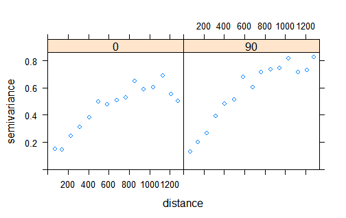
library(gstat)
library(sp)
data(meuse)
coordinates(meuse) = ~x+y
data(meuse.grid)
gridded(meuse.grid) = ~x+y

variog<-variogram(log(zinc)~1, meuse, width=90, cutoff=1300, alpha=c(0,90))
variog_map<-variogram(log(zinc)~1, meuse, width=90, cutoff=1300, map=T)
mydata<-data.frame(variog_map)

My data is what generates this figure

And i want to replicate this:

I copy below a question I asked on StackGIS. As it did not receive attention and may be asking about a bug, I thought I could post it here (sorry if it is not the case).
https://gis.stackexchange.com/questions/295213/cokriging-zero-distance-cross-semivariance-in-undersampled-cases-gstat-error

Trying to cokrige two variables that are not perfectly colocated (one has sparser measurements than the other), I faced an issue that I'll illustrate with the following MRE.

With the meuse dataset, consider we krige lead as principal variable assisted by copper measurements as auxiliary variable. We subset the lead, to simulate sparser measurements and hence, a need for cokriging with the denser copper measurements:

library("gstat")
library("sp")
data("meuse")
coordinates(meuse) = ~x+y

g <- gstat(NULL, data=meuse[1:80,], formula=lead ~ 1) # subset
g <- gstat(g, data=meuse, formula=copper ~ 1)
v <- variogram(g)
plot(v) # zero distance semivariance dot in panel var1.var2
g <- fit.lmc(v=v, g, vgm("Sph")) # error

You can see in the bottom-left panel of the plot a zero distance dot, which subsequently causes fit.lmc() to fail.

Now, if no subset is done (somewhat limiting the interest of cokriging, no?), everything works fine. This because, the zero distance dot in the cross-semivariogram does not appear in this case:

g <- gstat(NULL, data=meuse, formula=lead ~ 1)
g <- gstat(g, data=meuse, formula=copper ~ 1)
v <- variogram(g)
plot(v) # no zero dist dot on var1.var2 panel
g <- fit.lmc(v=v, g, vgm("Sph")) # fit fine with default fit.method

There is no reason for this dot to appear only in the subsetted cases, right?

Another example of this can be seen in this 2009 exercise document by Edzer Pebesma. In section 8.13, he refers to this as the "undersampled case". But the provided code is not working any more, likely for the reason mentioned above.

Thinking that undersampled cases are dealt with pseudo cross-vraiogram, I tried to play with parameter pseudo of variogram() but without success.

Is there is a simple way around this (hopefully) temporary bug?

Dear Edzer,

First of all I must congratulate you for the good job you did with the gstat package. It is amazing! :D

I am an Aerospace PhD candidate enrolled at the Technical University of Catalonia (UPC), and I am using gstat to model weather maps from aircraft meteorological reports (we have a lot).

I have started with the temperature (TAU) but the idea is to also model winds and pressure. My coordinates are latitude (LAT), longitude (LON) and altitude (H) (3D). I model the temperature as having a linear trend with H. Both LAT, LON and H are in meters.

Taking very consecutive messages (in a time window of 1 hour approximately) and using Universal kriging it works fine and results are very good!

However, I wanted to add the temporal dependence, since a recent aircraft report should have more “weight” than an older one.

I followed the instructions given by: https://www.r-bloggers.com/spatio-temporal-kriging-in-r/ but I am obtaining strange results.

I will show you what I get using variogram(TAUH, meteo,...)* and when I use variogramST(TAUH, timeDF,...)*. In this example I am using few data, but results are similar when using more than 6000 reports in a time window of 3 hours.

variogram(TAU~H, meteo,...)*
np dist gamma dir.hor dir.ver id
1 912 4228.952 0.7479942 0 0 var1
2 166 13008.030 1.9128943 0 0 var1
3 1 31536.365 0.1444785 0 0 var1
4 163 38952.849 1.0552677 0 0 var1
5 882 48600.833 2.6347495 0 0 var1
6 204 56619.013 6.3883626 0 0 var1
7 352 69922.614 1.3544736 0 0 var1
8 211 78979.202 2.0872938 0 0 var1
9 526 90706.807 2.5869795 0 0 var1

As I said, I am using few data. But using 6000 points the sill is 4 k^2 approximately and the range 30Km, with a clearly spherical behavior.

variogramST(TAU~H, timeDF,…)*
np dist gamma id timelag spacelag avgDist
1 32 224.3289 504.5851960 lag1 2.5 1000 358.4079
2 40 2938.8774 383.3689045 lag1 2.5 3000 2982.8571
3 40 4735.5115 260.1138000 lag1 2.5 5000 4799.4551
4 14 7054.1156 311.7253580 lag1 2.5 7000 6945.2808
5 10 8210.0676 23.2213242 lag1 2.5 9000 8253.3222
6 NA NA NA lag1 2.5 11000 11021.2858
7 NA NA NA lag1 2.5 13000 NaN

As you can see, the semivariance is much more large when using variogramST. I noticed that
variogramST(TAUH, timeDF,…) and variogramST(TAU1, timeDF,…) give me exactly the same result. Therefore the reason may be that variogramST is not taking tino account the trend of TAU with H, although H is a coordinate of the SpatialPoint object of timeDF :S

I checked all the variables and they have exactly the same structure that in the example provided by r-bloggers. I am sure that the problem is not the number of data points used to compute the variance for each time/distance lag, since with 6000 points differences between variogram and variogramST are still very large.

Do you have any clues about what is happening?

Thank you in advance and kind regards, :)

*meteo is a SpatialPointsDataFrame, timeDF is an object of class STIDF.

In the latest gstat version(1.1-4), fit.variogram appears to have become much less reliable even when fitting well-formed empirical variograms. In the example below, gstat 1.1-4 will produce a singular model warning. In contrast, if the same code is run under gstat 1.1-3, the variogram is fit without issue.

library(sp)
data(meuse)
coordinates(meuse) = ~x+y
vgm1 <- variogram(log(zinc)~1, meuse)
fit.variogram(vgm1, vgm("Sph"))

When doing a local space-time kriging, I see the message Using the following time unit: hours repeated thousands of times. This should be reduce to ... one?