The goal of the climate R package is to automatize downloading of meteorological and hydrological data from publicly available repositories:

• OGIMET (ogimet.com)
• University of Wyoming - atmospheric vertical profiling data (http://weather.uwyo.edu/upperair/).
• Polish Institute of Meterology and Water Management - National Research Institute (IMGW-PIB)
• National Oceanic & Atmospheric Agency - Earth System Research Laboratory - Global Monitoring Division (NOAA)

The stable release of the climate package from the CRAN reposity can be installed with:

install.packages("climate")

It is highly recommended to install the most up-to-date development version of climate from GitHub with:

library(remotes)
install_github("bczernecki/climate")

• meteo_ogimet() - Downloading hourly and daily meteorological data from the SYNOP stations available in the ogimet.com collection. Any meteorological (aka SYNOP) station working under the World Meteorological Organizaton framework after year 2000 should be accessible.

• meteo_imgw() - Downloading hourly, daily, and monthly meteorological data from the SYNOP/CLIMATE/PRECIP stations available in the danepubliczne.imgw.pl collection. It is a wrapper for meteo_monthly(), meteo_daily(), and meteo_hourly() from the imgw package.

• sounding_wyoming() - Downloading measurements of the vertical profile of atmosphere (aka rawinsonde data)

• meteo_noaa_co2() - Downloading monthly CO2 measurements from Mauna Loa Observatory

• hydro_imgw() - Downloading hourly, daily, and monthly hydrological data from the SYNOP / CLIMATE / PRECIP stations available in the danepubliczne.imgw.pl collection. It is a wrapper for hydro_annual(), hydro_monthly(), and hydro_daily() from the imgw package.

• stations_ogimet() - Downloading information about all stations available in the selected country in the Ogimet repository
• nearest_stations_ogimet() - Downloading information about nearest stations to the selected point available for the selected country in the Ogimet repository
• imgw_meteo_stations - Built-in metadata from the IMGW-PIB repository for meteorological stations, their geographical coordinates, and ID numbers
• imgw_hydro_stations - Built-in metadata from the IMGW-PIB repository for hydrological stations, their geographical coordinates, and ID numbers
• imgw_meteo_abbrev - Dictionary explaining variables available for meteorological stations (from the IMGW-PIB repository)
• imgw_hydro_abbrev - Dictionary explaining variables available for hydrological stations (from the IMGW-PIB repository)

library(climate)
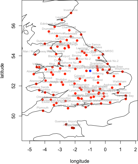
# find 100 nearest UK stations to longitude 1W and latitude 53N :

nearest_stations_ogimet(country = "United+Kingdom",
  date = Sys.Date(),
  add_map = TRUE,
  point = c(-1, 53),
  no_of_stations = 100
)

#     wmo_id                   station_names       lon      lat alt distance [km]
# 66   03354      Nottingham Weather Centre  -1.250005 53.00000 117      28.04973
# 69   03379                       Cranwell  -0.500010 53.03333  67      56.22175
# 68   03377                     Waddington  -0.516677 53.16667  68      57.36093
# 67   03373                       Scampton  -0.550011 53.30001  57      60.67897
# 78   03462                      Wittering  -0.466676 52.61668  84      73.68934
# 89   03544                 Church Lawford  -1.333340 52.36667 107      80.29844
# ...

library(climate)
o = meteo_ogimet(date = c(Sys.Date() - 5, Sys.Date() - 1), 
                 interval = "daily",
                 coords = FALSE, 
                 station = 12330)
head(o)

#>   station_ID       Date TemperatureCAvg TemperatureCMax TemperatureCMin TdAvgC HrAvg WindkmhDir
#> 3      12330 2019-12-21             8.8            13.2             4.9    5.3  79.3        SSE
#> 4      12330 2019-12-20             5.4             8.5            -1.2    4.5  92.4        ESE
#> 5      12330 2019-12-19             3.8            10.3            -3.0    1.9  89.6         SW
#> 6      12330 2019-12-18             6.3             9.0             2.2    4.1  84.8          S
#> 7      12330 2019-12-17             4.9             7.6             0.3    2.9  87.2        SSE
#>   WindkmhInt WindkmhGust PresslevHp Precmm TotClOct lowClOct SunD1h VisKm SnowDepcm PreselevHp
#> 3       11.4        39.6      995.9    1.8      3.6      2.0    6.7  21.4      <NA>         NA
#> 4       15.0          NA     1015.0    0.0      6.4      0.6    1.0   8.0      <NA>         NA
#> 5        7.1          NA     1020.4    0.0      5.2      5.9    2.5  14.1      <NA>         NA
#> 6        9.2          NA     1009.2    0.0      5.7      2.7    1.4  12.2      <NA>         NA
#> 7        7.2          NA     1010.8    0.1      6.2      4.6   <NA>  13.0      <NA>         NA

m = meteo_imgw(interval = "monthly", rank = "synop", year = 2000, coords = TRUE)
head(m)
#>            rank        id        X        Y   station   yy mm tmax_abs
#> 575 SYNOPTYCZNA 353230295 23.16228 53.10726 BIAŁYSTOK 2000  1      5.3
#> 577 SYNOPTYCZNA 353230295 23.16228 53.10726 BIAŁYSTOK 2000  2     10.6
#> 578 SYNOPTYCZNA 353230295 23.16228 53.10726 BIAŁYSTOK 2000  3     14.8
#> 579 SYNOPTYCZNA 353230295 23.16228 53.10726 BIAŁYSTOK 2000  4     27.8
#> 580 SYNOPTYCZNA 353230295 23.16228 53.10726 BIAŁYSTOK 2000  5     29.3
#> 581 SYNOPTYCZNA 353230295 23.16228 53.10726 BIAŁYSTOK 2000  6     32.6
#>     tmax_mean tmin_abs tmin_mean t2m_mean_mon t5cm_min rr_monthly
#> 575       0.4    -16.5      -4.5         -2.1    -23.5       34.2
#> 577       4.1    -10.4      -1.4          1.3    -12.9       25.4
#> 578       6.2     -6.4      -1.0          2.4     -9.4       45.5
#> 579      17.9     -4.6       4.7         11.5     -8.1       31.6
#> 580      21.3     -4.3       5.7         13.8     -8.3        9.4
#> 581      23.1      1.0       9.6         16.6     -1.8       36.4

h = hydro_imgw(interval = "semiannual_and_annual", year = 2010:2011)
head(h)
            id station riv_or_lake  hyy idyy Mesu idex   H beyy bemm bedd behm
3223 150210180 ANNOPOL   Wisła (2) 2010   13    H    1 227 2009   12   19   NA
3224 150210180 ANNOPOL   Wisła (2) 2010   13    H    2 319   NA   NA   NA   NA
3225 150210180 ANNOPOL   Wisła (2) 2010   13    H    3 531 2010    3    3   18
3226 150210180 ANNOPOL   Wisła (2) 2010   14    H    1 271 2010    8   29   NA
3227 150210180 ANNOPOL   Wisła (2) 2010   14    H    1 271 2010   10   27   NA
3228 150210180 ANNOPOL   Wisła (2) 2010   14    H    2 392   NA   NA   NA   NA

library(climate)
library(dplyr)

df = meteo_imgw(interval = 'monthly', rank='synop', year = 1991:2019, station = "POZNAŃ") 
df2 = select(df, station:t2m_mean_mon, rr_monthly)

monthly_summary = df2 %>% 
  group_by(mm) %>% 
  summarise(tmax = mean(tmax_abs, na.rm = TRUE), 
            tmin = mean(tmin_abs, na.rm = TRUE),
            tavg = mean(t2m_mean_mon, na.rm = TRUE), 
            opad = sum(rr_monthly) / n_distinct(yy))            

monthly_summary = as.data.frame(t(monthly_summary[, c(5,2,3,4)])) 
monthly_summary = round(monthly_summary, 1)
colnames(monthly_summary) = month.abb
print(monthly_summary)

#        Jan   Feb  Mar  Apr  May  Jun  Jul  Aug  Sep  Oct  Nov   Dec
# opad  37.1  31.3 38.5 31.3 53.9 60.8 94.8 59.6 40.5 39.7 35.7  38.6
# tmax   8.7  11.2 17.2 23.8 28.3 31.6 32.3 31.8 26.9 21.3 14.3   9.8
# tmin -15.0 -11.9 -7.6 -3.3  1.0  5.8  8.9  7.5  2.7 -2.4 -5.2 -10.4
# tavg  -1.0   0.5  3.7  9.4 14.4 17.4 19.4 19.0 14.3  9.1  4.5   0.8

# create plot with use of the "climatol" package:
climatol::diagwl(monthly_summary, mlab = "en", est = "POZNAŃ", alt = NA, 
  per = "1991-2019", p3line = FALSE)

  library(climate)
  co2 <- meteo_noaa_co2()
  head(co2)
  plot(co2$yy_d, co2$co2_avg, type='l')

Ogimet.com, University of Wyoming, and Institute of Meteorology and Water Management - National Research Institute (IMGW-PIB), National Oceanic & Atmospheric Agency, Earth System Research Laboratory, Global Monitoring Division (NOAA) are the sources of the data.

Contributions to this package are welcome. The preferred method of contribution is through a GitHub pull request. Feel also free to contact us by creating an issue.

To cite the climate package in publications, please use this paper:

Czernecki, B.; Głogowski, A.; Nowosad, J. Climate: An R Package to Access Free In-Situ Meteorological and Hydrological Datasets for Environmental Assessment. Sustainability 2020, 12, 394. https://doi.org/10.3390/su12010394"

LaTeX/BibTeX version can be obtained with:

library(climate)
citation("climate")