Provides the code to implement additive and multiplicative decompositoin model to monthly time series for forecast, testing and visualisation.

The decomposition model decomposes a time series into serveal components. Typically, they are trend component, seasonal component, cycle component and residual. In this work, only trend, seasonal, and residual components are considered. Cycle component is very hard to be generalised. The trend component is estimated by a polynominal regression of a chosen order. If order is 1, it is a linear regression.

Additive decomposition model: X_t = T_t + S_t + e_t

Multiplicative decomposition model: X_t = T_t * S_t * e_t

The suitable time series dataset for decomposition model is evenly-spaced data with seasonal pattern. The prediction is normally for short and medium term to aviod the trend component to explode.

Compared with more advanced predictive models for (evenly-spaced) time series problems, such as Holt-Winters and ARIMA, decomposition model provides more intuitive prospect for analysis. For most time series with regular seasonality, decomposition model is no worse than more advanced models.

Walkthough with Australian tourists data.

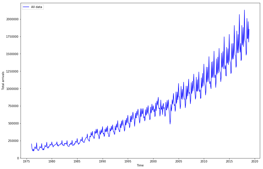
Original data

Decomposed components

Final prediction

Sample demonstration:

import decomposition

mdl_additive = decomposition.decomposition_additive()
mdl_multiplicative = decomposition.decomposition_multiplicative()

# Training and testing
mdl_additive.fit(train)
test_pred = mdl_additive.test(test)

# Prediction 
prediction = mdl_additive.predict(months = 36)