Git Product home page Git Product logo

miniufo / xinvert Goto Github PK

View Code? Open in Web Editor NEW
35.0 4.0 14.0 245.73 MB

Invert geophysical fluid dynamic problems (elliptic partial differential equations) using SOR iteration method.

Home Page: https://xinvert.readthedocs.io/

License: MIT License

Python 97.70% TeX 2.26% Shell 0.03%
successive-over-relaxation inversion-problem atmospheric-science oceanography meteorology omega-equation gill-matsuno-model munk-stommel wind-driven-circulation eliassen-model

xinvert's Introduction

xinvert

DOI GitHub Documentation Status PyPI version Workflow pytest Build Status status

animate plot

1. Introduction

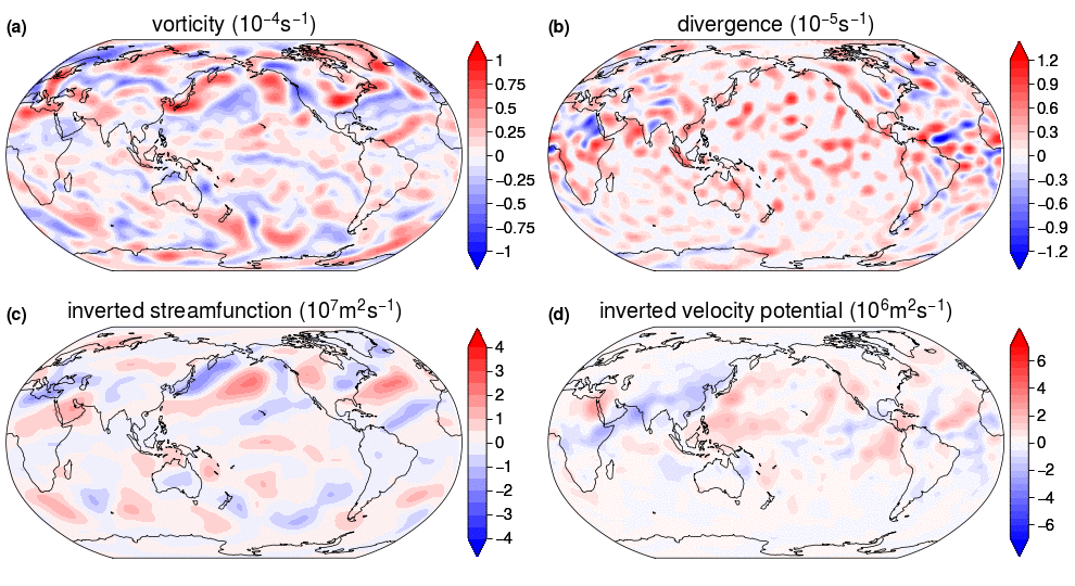
Researches on meteorology and oceanography usually encounter inversion problems that need to be solved numerically. One of the classical inversion problem is to solve Poisson equation for a streamfunction $\psi$ given the vertical component of vorticity $\zeta$ and proper boundary conditions.

$$\nabla^2\psi=\zeta$$

Nowadays xarray becomes a popular data structure commonly used in Big Data Geoscience. Since the whole 4D data, as well as the coordinate information, are all combined into xarray, solving the inversion problem become quite straightforward and the only input would be just one xarray.DataArray of vorticity. Inversion on the spherical earth, like some meteorological problems, could utilize the spherical harmonics like windspharm, which would be more efficient using FFT than SOR used here. However, in the case of ocean, SOR method is definitely a better choice in the presence of irregular land/sea mask.

More importantly, this could be generalized into a numerical solver for elliptical equation using SOR method, with spatially-varying coefficients. Various popular inversion problems in geofluid dynamics will be illustrated as examples.

One problem with SOR is that the speed of iteration using explicit loops in Python will be e-x-t-r-e-m-e-l-y ... s-l-o-w! A very suitable solution here is to use numba. We may try our best to speed things up using more hardwares (possibly GPU).

Classical problems include Gill-Matsuno model, Stommel-Munk model, QG omega model, PV inversion model, Swayer-Eliassen balance model... A complete list of the classical inversion problems can be found at this notebook.

Why xinvert?

  • Thinking and coding in equations: User APIs are very close to the equations: unknowns are on the LHS of =, whereas the known forcings are on its RHS;
  • Genearlize all the steady-state problems: All the known steady-state problems in geophysical fluid dynamics can be easily adapted to fit the solvers;
  • Very short parameter list: Passing a single xarray forcing is enough for the inversion. Coordinates information is already encapsulated.
  • Flexible model parameters: Model paramters can be either a constant, or varying with a specific dimension (like Coriolis $f$), or fully varying with space and time, due to the use of xarray's broadcasting capability;
  • Parallel inverting: The use of xarray, and thus dask allow parallel inverting, which is almost transparent to the user;
  • Pure Python code for C-code speed: The use of numba allow pure python code in this package but native speed;

2. How to install

Requirements xinvert is developed under the environment with xarray (=version 0.15.0), dask (=version 2.11.0), numpy (=version 1.15.4), and numba (=version 0.51.2). Older versions of these packages are not well tested.

Install via pip

pip install xinvert

Install from github

git clone https://github.com/miniufo/xinvert.git
cd xinvert
python setup.py install

3. Examples:

This is a list of the problems that can be solved by xinvert:

Gallery Gallery

invert Poisson equation for
horizontal streamfunction

invert Poisson equation for
overturning streamfunction

invert geostrophic equation for
balanced mass

invert Eliassen model for
overturning streamfunction

invert PV balance equation for
steady reference state

invert Gill-Matsuno model for
wind and mass fields

invert Stommel-Munk model for
wind-driven ocean circulation

invert Fofonoff model for
inviscid/adiabatic steady state

invert Bretherton model for
steady flow over topography

invert Omega equation for
QG vertical velocity

4 Animate the convergence of iteration

One can see the whole convergence process of SOR iteration as:

from xinvert import animate_iteration

# output has 1 more dimension (iter) than input, which could be animated over.
# Here 40 frames and loop 1 per frame (final state is after 40 iterations) is used.
psi = animate_iteration(invert_Poisson, vor, iParams=iParams,
                        loop_per_frame=1, max_frames=40)

See the animation at the top.

5 Cite

If you use the package in research, teaching, or other activities, we would be grateful if you mention xinvert and cite our paper in JOSS:

@article{Qian2023,
    doi = {10.21105/joss.05510},
    url = {https://doi.org/10.21105/joss.05510},
    year = {2023},
    publisher = {The Open Journal},
    volume = {8},
    number = {89},
    pages = {5510},
    author = {Yu-Kun Qian},
    title = {xinvert: A Python package for inversion problems in geophysical fluid dynamics}, journal = {Journal of Open Source Software}
}

xinvert's People

Contributors

damienirving avatar jbytecode avatar miniufo avatar navidcy avatar noraloose avatar

Stargazers

 avatar  avatar  avatar  avatar  avatar  avatar  avatar  avatar  avatar  avatar  avatar  avatar  avatar  avatar  avatar  avatar  avatar  avatar  avatar  avatar  avatar  avatar  avatar  avatar  avatar  avatar  avatar  avatar  avatar  avatar  avatar  avatar  avatar  avatar  avatar

Watchers

 avatar  avatar  avatar  avatar

xinvert's Issues

add a Fofonoff model

Fofonoff (1954) proposed a nonlinear steady-state solution of an ocean, with an initial energy but no forcing and dissipation (conservative flow). This model fits the solver well.

invert_omega: Need to pass N2 and f0 as dataArrays

Hi,

Is it possible to pass different values of N2 per pressure level, and f0 per latitude, in the form of coordinate-aware arrays? In particular, N2 is quite different for the upper and lower levels.

Thanks!

JOSS review: Automated tests

@miniufo - well done on your submission to JOSS.

As it stands, your package doesn't meet the following requirement on the reviewer checklist:

Automated tests: Are there automated tests or manual steps described so that the functionality of the software can be verified?

(See openjournals/joss-reviews#5510 for details.)

You've got some test code available at tests/ and associated data files at Data/, but there is no guidance provided on how to run those tests manually or better still there is no automated testing.

In addition, it looks like your test code culminates in the plotting of figures. While that can be useful for visual verification, common practice would also include a suite of tests that have the following components:

  • a fixture, which is the thing being tested (e.g., an input data array);
  • an actual result, which is what the xinvert package produces when given the fixture; and
  • an expected result that the actual result is compared to.

The comparison between the actual result and expected result would take the form of an assertion, so that the test can be said to pass or fail. You can then use a test runner like pytest in conjunction with GitHub actions to setup automated testing.

You may already be familiar with these testing concepts, but if not let me know and I can point you to some resources that explain how to setup automated testing.

refactor of the internal API

As I want to fit more problems into the architecture of xinvert, the current design of this package makes it a bit hard for some problems. Specifically, it is much better to refactor the internal design of this package, and also change the user APIs accordingly. Specifically, the problems are:

  • Too many keyword arguments in a single problem. It is best to separate these kwargs into two kinds: one is model parameters mParams that prescribed in the model or equation. For example, Coriolis paramter $f$ and stratification $N^2$. The other kind is invert paramters iParams that controls the iteration and has nothing to do with the model. For example, maximum loops or tolerance for stop looping.
  • Sometimes the required model parameters are less than the coefficients of the equation. But calculating the coefficients requires finite difference capability. This original depends on xgcm. However, xgcm is still in heavy development and is targeted at Arakawa C-grid. Since I don't want this package to be fully relied on xgcm, I need to add this finite difference capability.
  • Animate the iteration should be generalized to accept every invert function. So we only need a single animate_iteration function fo all the models.
  • Gill-Matsuno model and Stommel-Munk model are found to be fitted into the standard model. Not sure if they should be solved using the standard solver or still using the general solver.

'dz' counts a lot

Hi,

I'm trying to use the method in a domain which has 19 levels in depth (totally 1000m), and I found it makes a poor inversion result. However, it comes a much better result after I set my vertical levels as the data used in oceanic example (200 levels for 1000m), which convinced me that 'dz' counts a lot in calculation. But with the improvement comes a fat data array ( [360,200,1700,650] ) that is so hard to run forward. So I’d like to know, from your perspective, what value of 'dz' (or levels in depth) can allows me to reduce the size of data while maintaining a good accuracy?

Thanks a lot!

add a 2D reference state example

Recently, I find that the steady state for 2D shallow-water model can be cast as a 2nd-order PDE that fits the solver. So just do it.

a constants module

xinvert uses many constants within the package. However, these constants need to be modified in some cases. For example, a numerical model may use 6371,000 as the radius of the earth, while here 6371,200 is used as default. We need to add a constants module, so that these constants can be modified by users across the whole package, based on their needs.

Parallel calculation using dask

Although the current implementation is based on xarray and dask. The solution is first loaded completely into memory. During the multi timesteps calculation, xinvert does not accelerate on a multi-core PC. This is a little strange to me and need some times to make it parallelable.

boundary conditions

Currently, the boundary conditions are specified as:

sf = invert_Poisson(vor, dims=['lat', 'lon'], BCs=['fixed', 'periodic'])

which means the north-south BCs are all fixed and east-west BCs are periodic. This is not flexible enough if one wants the north BC as the 'fixed' one while the south BC as the 'extend' or 'reflect' one.

One possible solution is to use dict to specify BCs as:

sf = invert_Poisson(vor, dims=['lat', 'lon'], BCs={'lat':('fixed'. 'extend'), 'lon':('periodic', 'periodic')})

Also, I am thinking if the underlying algorithm should be refactored as two steps: 1) pad the domain with proper BCs and 2) iterate for the solution. But this may cause some problems if BCs are at 1) poles and 2) vortex center where coordinates are undefined.

JOSS review: Installation

@miniufo - well done on your submission to JOSS.

As part of my review of your submission (see openjournals/joss-reviews#5510), I have some questions/suggestions regarding software installation:

  • In the "how to install" (https://github.com/miniufo/xinvert#2-how-to-install) section of your README file it says "install via pip (not yet)" but as far as I can tell it can be installed by pip. What is the meaning of "not yet"?
  • Do you think it would be advantageous to also make the package available via conda (i.e. conda-forge) for users who manage their python environments using conda?

add a example of Bretherton-Haidvogel model for 2D turbulence over topography

This is an example I recently ran into, which adopted a variational calculas to get the steady-state equation between a 2D flow with total kinetic energy $E_0$ and a given topography (small compared with fluid depth).

Once the topography is specified, the steady state of the flow with $E_0$ is also determined.

Diabatic Forcing term in QG Omega

The Q-vector form of the Omega equation doesn't have an adiabatic forcing term in your calculation. Is there any easy way to incorporate that term while calculating the Omega value from the Qvector form of the Omega equation?

Extrapolation of results beyond the heating source

Hi, I've run xinvert for the Gill-Matsuno problem over the maritime continent, as shown in your example. The results I've got regarding h1, u1 and v1 are constrained just to the heating source region (see attached figure), but not to the entire Indo-Pacific region as in your figures. I think the problem can be in the plotting of the wind and streamfunction, which I include below. I appreciate any help. Many thanks in advance.

##########################
import os
import matplotlib.pyplot as plt
from netCDF4 import Dataset as netcdf_dataset
import numpy as np

from cartopy import config
import cartopy.crs as ccrs
import cartopy.feature as cfeature
from cartopy.mpl.ticker import (LongitudeFormatter, LatitudeFormatter,
LatitudeLocator)

plt.figure(figsize=(40,20))

heat = Q1
lats = lat
lons = lon

skip = 1
fontsize = 16

ax = plt.axes(projection=ccrs.PlateCarree())
ax.coastlines()
ax.add_feature(cfeature.BORDERS)
Results constrained to Heating Source Region

Grid for Heating source - Maritime Continent

ax.gridlines(crs=ccrs.PlateCarree(), draw_labels=True,
xlocs=np.arange(-140,100, 80), ylocs=np.arange(-40, 40, 40),
x_inline=False, y_inline=False, linewidth=0.33, color='k',alpha=0.5)

Heat Source Region

cmap = plt.colormaps['jet']
ax.contourf(lons, lats, Q1, 10, transform=ccrs.PlateCarree(), cmap=cmap , levels=np.linspace(-0.05, 0.05, 10))

Contours for h1

ax.contour(lons, lats, h1, transform=ccrs.PlateCarree(), cmap='jet')

windspeed = (u1 ** 2 + v1 ** 2) ** 0.5
windspeed.rename('windspeed')

Plot the wind speed as a contour plot

ax.contour(lons, lats, windspeed, 20, cmap='jet')

Add arrows to show the wind vectors

plt.quiver(lons, lats, u1, v1, pivot='middle', width=0.0015, headwidth=1., headlength=1., minlength=1)

#Limits for Maritime Continent
Results constrained to Heating Source Region

ax.set_ylim([-40, 40])
ax.set_xlim([40, 200])

plt.show()

QG Omega

Hi, I am trying to reproduce the vertical velocity using QG Omega inversion. If I need to invert the equation for the western hemisphere only, how do I need to change the boundary conditions?

add a vertical mode decomposition case

Vertical mode decomposition (VMD) is a common way to analyze the vertical structure of many phenomena. Generally, given a vertical profiles of $N^2$ at a single point, it is able to project any variable onto a series of vertical modes determined by $N^2$. It should be 1D problem along the z coordinate.

Dependence on xcontour package

I'm opening a new issue here to continue the discussion on the issue of the xcontour dependence that we started here.

The dependence of xcontour is a bit complicated. It is another package I've written here. So the example of reference state, which is newly added, depends on xcontour to prepare the forcing (actually preparing the forcing data is not the core part of xinvert). This is not necessary for other examples. So far, I don't have any plan to get xcontour released as a conda package, so it is not possible to add this to conda dependency. Do you have any suggestion? I really like this example to remain in the problem list.

Is there a way to precompute M(Q) and C(Q) with xcontour and in the https://xinvert.readthedocs.io/en/latest/notebooks/05_reference_SWM.html example, and just load these states from netcdf if xcontour is not available? You could then adapt the notebook as follows:

try:
    import xcontour
    # do xcontour computation in this notebook, as you do now
except ImportError:
    ds = xr.open_dataset(your_precomputed_dataset)

This is part of the review process at openjournals/joss-reviews#5510.

JOSS review: community guidelines

@miniufo - well done on your submission to JOSS.

As it stands, your package doesn't meet the following requirement on the reviewer checklist:

Community guidelines: Are there clear guidelines for third parties wishing to 1) Contribute to the software 2) Report issues or problems with the software 3) Seek support

(See openjournals/joss-reviews#5510 for details.)

JOSS review: state of the field

@miniufo - well done on your submission to JOSS.

There is a requirement on the reviewer checklist relating to the software paper which reads as follows:

State of the field: Do the authors describe how this software compares to other commonly-used packages?

(See openjournals/joss-reviews#5510 for details.)

You make a comparison against windspharm in your README file...

Inversion on the spherical earth, like some meteorological problems, could utilize the spherical harmonics like windspharm, which would be more efficient using FFT than SOR used here. However, in the case of ocean, SOR method is definitely a better choice in the presence of irregular land/sea mask.

... but not in the software paper itself. I think it would be worth mentioning windspharm (and any other relevant commonly-used packages) in your software paper too.

Lat-Lon Finite Differences

Hi, this package looks really neat!

I was wondering if you had a reference for how you are calculating the finite differences with spherical coordinates? From the looks of it, you’re simply multiplying the Y-axis by a scalar factor of degrees to meters and the X-axis by the same plus and a cosine of the Y-coords. I’m not familiar with this but this seems really, really useful in general with finite differences for lat-lon.

Do you have a reference or something I could look at because I’m not familiar with this but I would really like to use it.

Thanks!

Pressure perturbation equation

Hello,
I'm working with the dynamic pressure perturbation equation (Laplacian of p = -roh*((dudx)**2+(dvdy)**2+(dwdz)**2)). At small scales, what boundary conditions, mxLoop, and tolerance would you reccomend?

A list of all the inverting problems

A summary table of all the current problems would be good for the users to see the functionality of xinvert. Also, such a table makes an example for the users and they can also add their own problems.

Can't reproduce QG example

Hello, I'm very new to python and trying to implement the QG omega test case using the sample data: atmos3D.nc provided, but I keep running into the following error upon executing the testOmegaEq.py script:

Traceback (most recent call last):
File "", line 1, in
File "", line 18, in
File "C:\Users\user-pc\miniconda3\Lib\site-packages\xinvert\tests\GeoApps\GridUtils.py", line 70, in add_latlon_metrics
dlonG = grid.diff(ds[lon ], 'X', boundary_discontinuity=360)
File "C:\Users\user-pc\miniconda3\lib\site-packages\xgcm\grid.py", line 2093, in diff
return self._1d_grid_ufunc_dispatch("diff", da, axis, **kwargs)
File "C:\Users\user-pc\miniconda3\lib\site-packages\xgcm\grid.py", line 1836, in _1d_grid_ufunc_dispatch
array = grid_ufunc(
File "C:\Users\user-pc\miniconda3\lib\site-packages\xgcm\grid_ufunc.py", line 460, in call
return apply_as_grid_ufunc(
File "C:\Users\user-pc\miniconda3\lib\site-packages\xgcm\grid_ufunc.py", line 770, in apply_as_grid_ufunc
results = _apply(
File "C:\Users\user-pc\miniconda3\lib\site-packages\xgcm\grid_ufunc.py", line 837, in _apply
results = xr.apply_ufunc(
TypeError: apply_ufunc() got an unexpected keyword argument 'boundary_discontinuity'

Can you please assist in figuring out what is causing this?

Re-running notebooks

When trying to re-run the notebooks, three of them fail:

  • In 11_Omega_equation.ipynb the following fails because the netcdf file is not available
ds = xr.open_dataset('I:/Omega/OFES30_20011206_Qian/data.nc',
                     chunks={'lev':6}).astype('f4')
  • In 04_Eliassen_model.ipynb the following fails:
ds = xr.open_dataset('../../../Data/Zonalmean.nc')

The latter is simply a typo in the filename; it needs to be changed to ./../../Data/ZonalMean.nc

  • In test_01_Stommel_Arons_model.ipynb the following fails:
eps = xr.where(basin, eps, np.nan)

with the error

ValueError: cannot align objects with join='exact' where index/labels/sizes are not equal along these coordinates (dimensions): 'lon' ('lon',)

This is part of the review process at openjournals/joss-reviews#5510.

Recommend Projects

  • React photo React

    A declarative, efficient, and flexible JavaScript library for building user interfaces.

  • Vue.js photo Vue.js

    🖖 Vue.js is a progressive, incrementally-adoptable JavaScript framework for building UI on the web.

  • Typescript photo Typescript

    TypeScript is a superset of JavaScript that compiles to clean JavaScript output.

  • TensorFlow photo TensorFlow

    An Open Source Machine Learning Framework for Everyone

  • Django photo Django

    The Web framework for perfectionists with deadlines.

  • D3 photo D3

    Bring data to life with SVG, Canvas and HTML. 📊📈🎉

Recommend Topics

  • javascript

    JavaScript (JS) is a lightweight interpreted programming language with first-class functions.

  • web

    Some thing interesting about web. New door for the world.

  • server

    A server is a program made to process requests and deliver data to clients.

  • Machine learning

    Machine learning is a way of modeling and interpreting data that allows a piece of software to respond intelligently.

  • Game

    Some thing interesting about game, make everyone happy.

Recommend Org

  • Facebook photo Facebook

    We are working to build community through open source technology. NB: members must have two-factor auth.

  • Microsoft photo Microsoft

    Open source projects and samples from Microsoft.

  • Google photo Google

    Google ❤️ Open Source for everyone.

  • D3 photo D3

    Data-Driven Documents codes.