For aspiring data scientists, like yourselves, regression analysis the first real "learning" algorithm that they come across with. It is one of the simplest algorithms to master but still requires some statistical understanding of the underlying. This lesson will introduce you to regression process based on the statistical ideas we have discovered so far.

You will be able to:

• Describe statistical modeling with simple regression
• Explain simple linear regression as solving for equation y=mx+c
• Calculate the slope and y-intercept using the slope value
• Draw a regression line based on calculated slope and intercept
• Predict the target of a previously unseen input feature

So far, we have covered topics like basic hypothesis testing, variable relationships, statistical learning. We shall now build on these ideas to explain the regression process. Regression is a parametric technique used to predict the value of a target variable Y based on one or more input feature variables X. Regression is proven to give credible results if the data follows parametric assumptions which will be covered in upcoming lessons. Regression Analysis helps us with analytics in following ways:

• Finding an association, relationship between variables.
• Identifying which variables contribute more towards the outcomes.

and most importantly ..

• Prediction of future observations.

As we saw in pevious lesson, linear implies that the model functions along a straight or nearly straight line. Linear suggests that the relationship between dependent and independent variable can be expressed in a straight line. A Simple Linear Regression uses a single feature (independent variable) to predict a target (dependent variable) by fitting a best linear relationship, whereas Multiple Linear Regression uses more than one features to predict a target variable by fitting a best linear relationship. In this section, we shall mainly focus on simple regression to build a sound understanding.

So let's move on and see how to calculate such a line.

We all know from elementary geometry that equation of a stright line can be written as:

Following what we have covered so far, we can say from the equation that:

• y is the dependent variable i.e. the variable that needs to be estimated and predicted.
• x is the independent variable i.e. the variable that is controllable. It is the input.
• m is the slope. It determines what will be the angle of the line. It is the parameter denoted as β.
• c is the intercept. A constant that determines the value of y when x is 0.

Linear regression is nothing but a manifestation of this simple equation. The formula for the best-fit line (or regression line) is still "a line".

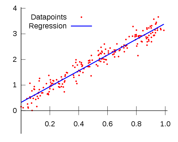
A model really cant get any simpler than this. This equation here is the same one used to find a line in algebra, but in statistics the points don’t lie perfectly on a line as shown above

The line is a model around which the data lie if a strong linear pattern exists.

Following image that we saw in previous lesson explains this further.

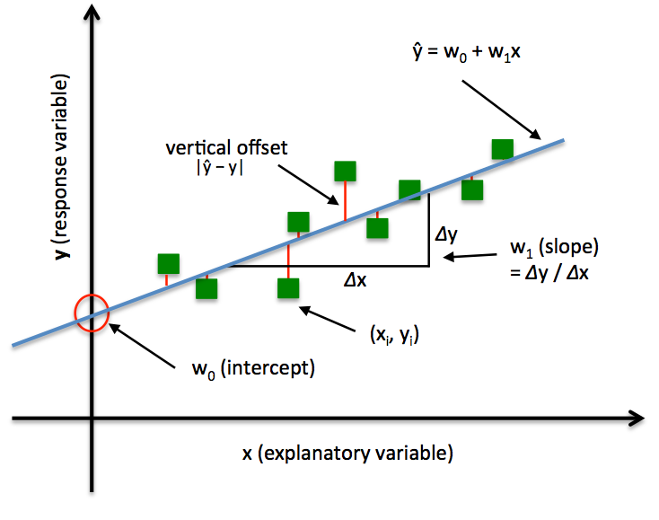
The slope (m) of a line is the change in Y over the change in X (Δy/Δx shown above). For example, a slope of 4/3 means as the x-value increases by 4 units, the y-value moves up by 3 units on average.

The y-intercept (b) is the value on the y-axis where the line crosses the axis. For example, in the equation y= 2x +2, the line crosses the y-axis at the value b = 2. The coordinates of this point would be (0, 2).

When a line crosses the y-axis, the x-value is always 0.

You may be thinking that you have to try lots and lots of different lines to see which one fits best. Fortunately, this task is not as complicated as in may seem . Given some data points, the best-fit line always has a distinct slope and y-intercept that can be calculated using simple linear algebraic approaches.

Before we calculate the best-fit line, we have to make sure that we have calculated following measures for variables x and y:

• The mean of the x (x_bar)

• The mean of the y (y_bar)

• The standard deviation of the x values (denoted Sx)

• The standard deviation of the y values (denoted Sy)

• The correlation between X and Y (denoted r - following Pearson Correlation)

The formula for the slope (shown as b below), of the best-fit line is

So You simply divide sy by sx and multiply the result by r.

The slope of the best-fit line can be a negative number following a negative correlation. For example, if an increase in police officers is related to a decrease in the number of crimes in a linear fashion, the correlation and hence the slope of the best-fitting line is negative in this case.

Slope is not same as correlation.Slope takes the untiless correlation and attaches units to it. Think of Sy divided by Sx as the variation (resembling change) in Y over the variation in X, in units of X and Y.

So now that we have slope value (b), we can put it back into our formula to calculate intercept (shown as a below).

x_bar and y_bar are the mean values for variables x and y. So to calculate the y-intercept of the best-fit line, you start by finding the slope of the best-fit line using the above steps. Then to find the y-intercept, you multiply slope value mean of x and subtract the result from mean of y.

Once we have a regression line with defined parameters - slope and intercept as shown above, We can easily predict the y_hat (target) value for a new x (feature) value using the parameter values:

Remember that the different between y and y_hat is that y_hat is the y value predicted by the fitted model, whereas y carries actual values of variable (called the truth values) that were used to calculated the best fit.

Next we shall move on and try to code these equations in to draw regression line to a simple dataset to see all of this in action.

In this lesson, we learnt the basics of simple linear regression between two variables as a problem of fitting a straight line to best describe the data associations on a 2-dimensional plane. Remember this is only half the process. Once we have coded these equations as functions, we shall move on to calculating the loss in our model.