Keywords: GWAS (Genome-wide Association Studies), Phenotype Simulation, PRS (Polygenic Risk Score), C+T (Clumping and Thresholding), BASIL (Lasso Regression), and BayesR (Bayesian Regression)

• Keng-Chi Chang
• Po-Chun Wu

Polygenic Risk Scores (PRS) hold promise for personalized medicine but face challenges in prediction accuracy. This study investigates how simulation parameters affect PRS accuracy using Clumping + Thresholding, BASIL (Lasso-based method in snpnet package), and BayesR (Bayesian Multiple Regression-based method in GCTB package). By manipulating parameters such as heritability, number of causal SNPs, and how minor allel frequency affects heritability, we aim to understand whether certain PRS method might have advantage over others, and under what conditions. Our findings can inform the selection of PRS and phenotype simulation methods for precise disease risk prediction in clinical and research settings, advancing personalized healthcare interventions.

• Clumping + Thresholding (C+T) (PLINK 2)
• Batch Screening Iterative Lasso (BASIL)
• Bayesian Multiple Regression (BayesR)

1. Since Clumping + Thresholding does not directly model the additive effects of the contribution from multiple SNPs, we expect that C+T would perform the worst when the number of causal SNPs increases.
2. Both BASIL and BayesR should be better at capturing additive effects from many SNPs, while shrinkage-based method might incorrectly shrink some effects to zero.

Consider heritability model of the form (Speed, Holmes, and Balding 2020) $$\mathbb{E}\left[h^2_j\right]=\sum_j w_j\left[f_j(1-f_j)\right]^{(1+\alpha)},$$ where $w_j$ is the weight for SNP $j$ and $f_j$ is its minor allele frequency (MAF). For simplicity, we assume that weight $w_j$ is a constant.

3. When $\alpha=-1$, the expected heritability reduces to $\sum_j w_j$. SNPs have linear effect on heritability, regardless of minor allele frequency. Since this data generating process is closer to Lasso, we expect BASIL to perform better under this regime.
4. When $\alpha=-0.25$, the expected heritability becomes $\sum_j w_j\left[f_j(1-f_j)\right]^{0.75}$. SNPs that are more common would have higher contribution to heritability. We expect BayesR would capture this nonlinear relationship better than Lasso based BASIL.

The current published papers comparing these methods have mixed findings. Most of them either only use simulated genotypes, simulate phenotypes on a narrow demography (Lloyd-Jones et al. 2019; Qian et al. 2020), or does not systematically evaluate alternative scenarios (Ding et al. 2023). To our knowledge, this is the first systematic comparison on real genomic data across ancestries/populations.

We are analyzing real genome data from 1000 Genomes Project Phase Three call set on GRCh37. Since the size of the data is huge, for the ease of data storage and collaborating, we store our data on Google Drive and use Google Colab for compute (by reading/copying files directly from Google Drive).

• Notes: We have updated the related notebooks and the data of calculation results on GitHub. However, due to the large size of other raw data, we have only placed it on Google Drive.

Here is the link to our Google Drive project folder.

GitHub Directory:

.
├── notebook                   ← Codes and scripts
├── data
│   ├── BASIL/chr19_ldl_pheno  ← Results of BASIL
│   ├── BayesR/chr19_ldl_pheno ← Results of BayesR
│   ├── CT/chr19_ldl_pheno     ← Results of C+T
│   ├── chr19_ldl_pheno        ← Simulated phenotypes
│   └── split_ids              ← Sample splitting (train, val, test)
│       ├── by_population
│       └── by_superpopulation 
└── figure                     ← Analysis and graphs

Part of the files in Google Drive Project are organized as follows:

/CSE-284-Final-Project/
├── data
│   ├── 1000g_by_superpopulation ← Genome (all autosomes) split by superpopulation
│   │   ├── AFR_{train,val,test}.{bed,bim,fam,pgen,pvar.zst,psam}
│   │   ⋮    ⋮
│   │   └── SAS_{train,val,test}.{bed,bim,fam,pgen,pvar.zst,psam}
│   ├── 1000g_by_population ← Genome (all autosomes) split by perpopulation
│   │   ├── ACB_all.{bed,bim,fam,pgen,pvar.zst,psam}
│   │   ⋮    ⋮
│   │   └── YRI_all.{bed,bim,fam,pgen,pvar.zst,psam}
│   ├── 1000g_combined ← Genome (all autosomes) 
│   │   └── 1000g.{bed,bim,fam,pgen,pvar.zst,psam}
│   ├── 1000g_raw_combined ← Raw genome before cleaning and quality control
│   │   ├── all_phase3.{pgen.zst,pvar.zst}
│   │   ├── phase3_corrected.psam
│   │   ├── raw.{bed,bim,fam}
│   │   └── clean.{bed,bim,fam}
│   ├── 1000g_pheno ← Simulated phenotype by parameters
│   │   └── power={-1,-0.25}_her={0.1,0.3,0.5,0.7,0.9}_num-causals={1,10,100,1000,10000}.phen
│   ├── igsr_samples.tsv ← Reference table for population and sex information
│   ├── split_samples.csv ← Reference table for sample splitting
│   ├── split_ids ← Ids after sample splitting (for `--keep`)
│   │   ├── by_superpopulation
│   │   └── by_population
│   └── test_data ← Genome and phenotype data for benchmark (from PS4)
│       ├── CEU_chr19_normed.{bed,bim,fam,pgen,pvar.zst,psam}
│       ├── GBR_chr19_normed.{bed,bim,fam,pgen,pvar.zst,psam}
│       └── kgvcf_ldl.{phe,phen,pheno}
└── notebook ← Data processing and analysis
    ├── 00_download_1000genome_data_and_simulate_phenotypes.ipynb
    ├── 01_convert_to_pgen.ipynb
    ├── 02_convert_to_bed.ipynb
    ├── 04_split_train_val_test.ipynb
    ├── 05_simulate_phenotype.ipynb
    ├── 06_update_phenotype_format.ipynb
    ├── 07_convert_chr19.ipynb
    ├── 08_LDAK_chr19_pheno_simulation.ipynb
    ├── 09_test_GCTA_pheno_simulation.ipynb
    ├── 11_test_snpnet.ipynb
    ├── 12_test_GCTB.ipynb
    ├── 13_test_C+T.ipynb
    ├── 21_1000g_snpnet.ipynb
    ├── 22_1000g_GCTB.ipynb
    ├── 23_1000g_CT_population.ipynb
    ├── 24_CT_test_PS4.ipynb
    ├── 31_snpnet_superpopulation.ipynb
    ├── 32_GCTB_superpopulation.ipynb
    ├── 33_CT_superpopulation.ipynb
    ├── 34_CT_population.ipynb
    ├── 41_chr19_prs_by_superpopulation_check_progress.ipynb
    ├── 42_chr19_prs_by_superpopulation_analysis.Rmd
    ├── 42_chr19_prs_by_superpopulation_analysis.html
    ├── 42_chr19_prs_by_superpopulation_analysis.md
    └── 43_analysis.ipynb

• File naming of notebook directory
  • 0x: Data Preprocessing
  • 1x: Model testing
  • 2x: Run models on all autosomes
  • 3x: Run models on Chr 19 only (final setting)
  • 4x: Results and analysis

• Goal: get the dataset of all autosomes from 1000 Genomes with quality control
• Tool: PLINK 1.9 and PLINK 2.0
• Data Quality Control
  • --maf 0.01 --snps-only just-acgt --max-alleles 2 --rm-dup exclude-all
• Convert to binary formats for different packages
  • For BASIL/snpnet: --make-pgen generates .pgen .pvar .psam
  • For BayesR/GCTB: --make-bed generates .bed .bim .fam
• Dataset
  • Raw data: data/1000g_raw_combined/
  • Cleaned data: data/1000g_combined/
  • Split by Population: data/1000g_by_population/
  • Split by Super-population: data/1000g_by_superpopulation/
• Reference: https://dougspeed.com/1000-genomes-project/

(Number of Samples from Each Superpopulation on 1000 Genomes Project Phase 3 Dataset)

• Goal: simulate phenotypes with different settings
• Tool: LDAK
• Options
  • --make-phenos: perform simulation
  • --power ($\alpha$) : specify how predictors are scaled
    • Diffirent from the power mentioned in the class that indicates the probability we can detect an association at the desired significance level, given that there is actually an association.
  • --her: heritability describes how much variation in the phenotype is described by genetics.
  • --num-phenos: the number of phenotypes to generate.
  • --num-causals: the number of predictors contributing to each phenotype.
  • --causals <causalsfile>: specify which predictors are causal for each phenotype.
  • --effects <effectsfile>: specify the effect sizes in a file.
• Our simulation settings
  • Number of Phenotypes: 20
  • Power: {-0.25, -1}
    • Notes: GCTA Model with power of -1 vs. Human Default Model with power of -0.25
  • Heritability: {0.1, 0.3, 0.5, 0.7, 0.9}
  • Number of causal SNPs = {1, 10, 100, 250, 512}
  • Total combinations: 2 * 5 * 5 = 50
  • File naming: power=x_her=y_num-causals=z.pheno
  • Columns: FID, IID, PHEN1, PHEN2, PHEN3, ...
• Notes: At first, we didn't specify the <causalsfile> and <effectsfile>. By default, LDAK will pick causal predictors at random and sample effect sizes from a standard normal distribution. However, the results of PRS using randomly selected causal SNPs and effect sizes are horrible ($R^2$ of testing data close to $0$). Therefore, we adopted the ldl_prs.txt data from UCSD CSE 284 PRS Activity, which is the LDL PRS data from this paper and its publicly available data. Also, since there are 512 SNPs on Chromosome 19 listed in ldl_prs.txt, the maximal number of causal SNPs is 512.
• Dataset
  • data/chr19_ldl_pheno/
• Reference: https://dougspeed.com/simulations/

• We randomly select samples from each superpopulation into 70% training, 15% validation, and 15% test sets, while keeping each set has balanced number of samples from each population and sex.

• Dataset
  • data/split_ids/
    • by_population/
    • by_superpopulation/

$$PRS_i = \sum_{j \in S} \beta_j X_{ij}$$

• Tool: PLINK 2.0
• Reference: UCSD CSE 284 Week 6 Lecture Slides, PS3, and PS4

1. Perform a GWAS to estimate per-variant effect sizes ($\beta$'s)
   • --linear --maf 0.05 $$Y = \beta_j X_j + \epsilon$$
2. Perform LD clumping (pruning) to get an independent set of SNPs
   • --clump gwas.assoc.linear
   • --clump-p1 0.0001: significance threshold for index SNPs
   • --clump-r2 0.1: LD threshold for clumping
   • –clump-kb 250: physical distance threshold for clumping
3. Choose all SNPs with $p$-value less than the threshold $T$
4. Computer PRS and evalueate accuracy ($R^2$)
   • --score
5. Computer final PRS with optimal $T$ and evaluate on a separate testing dataset

• Repeat steps 2-4 to find out which $T$ work the best (validation dataset)
• Notes: When running C+T for AMR (superpopulation) dataset from 1000 Genomes, we encountered a problem that PLINK 2.0 will not run the --score command when there are less than 50 samples. Since there are not enough samples for validation data. We choose the best p value threhold $T$ in the training data as the $T$ for testing data. Thus, the performance may be underrated.

$$\mathrm{Minimize} \sum_i (y_i - \hat{y}_i)^2 + \lambda \sum_j |\hat{\beta}_j|$$

• Tool: snpnet
• Reference: Vignette of the snpnet R package by Junyang Qian and Trevor Hastie

1. (Already preprocessed) convert genotypes to .pgen
2. Train snpnet() model, get fit_snpnet object in R

• niter = 100 controls the number of iterations
• use.glmnetPlus = TRUE recommended for faster computation

3. Predict phenotype using predict_snpnet(), get pred_snpnet object

• fit = fit_snpnet to use the fitted model
• new_genotype_file to test on test set

4. Evaluate $R^2$ in pred_snpnet$metric

• Tool: GCTB
• Reference: Tutorial: Practical 4 Bayesian methods for genomic prediction by GCTB package maintainer Jian Zeng

1. (Already preprocessed) convert genotypes to .bed
2. Train BayesR model

• --chain-length 10000 controls total length of Markov Chain
• --burn-in 2000 controls number of burn-ins

3. Get posterior effects for each SNP in .snpRes format
4. Send .snpRes to plink for scoring of PRS scores
5. Calculate $R^2$ against the ground truth

• $R^2$ of testing data close to $0$ 🥲
• Probably because there are not enough samples to model the complicated relaitonships between variants and phenotypes.

• $R^2$ of testing data close to $0$ 🥲
• Probably because there are not enough samples to model the complicated relaitonships between variants and phenotypes.

• It works 😃
  • Superpopulation: {'AFR', 'AMR', 'EAS', 'EUR', 'SAS'}
  • Power: {-0.25, -1}
  • Heritability: {0.1, 0.3, 0.5, 0.7, 0.9}
  • Number of causal SNPs = {1, 10, 100, 250, 512}
  • Output files
    • combined_predict_{superpopulation}_power={power}_her={heritability}_num-causals={number of causal SNPs}_pheno={number of phenotypes}.csv
      • Columns: IID, Predicted Phenotype, Actual Phenotype, Phenotype Index
    • combined_result_{superpopulation}_power={power}_her={heritability}_num-causals={number of causal SNPs}_pheno={number of phenotypes}.csv
      • Columns: Superpopulation, Power, Heritability, Number of Causal SNPs, Phenotype Index, Training $R^2$, Validation $R^2$, Testing $R^2$

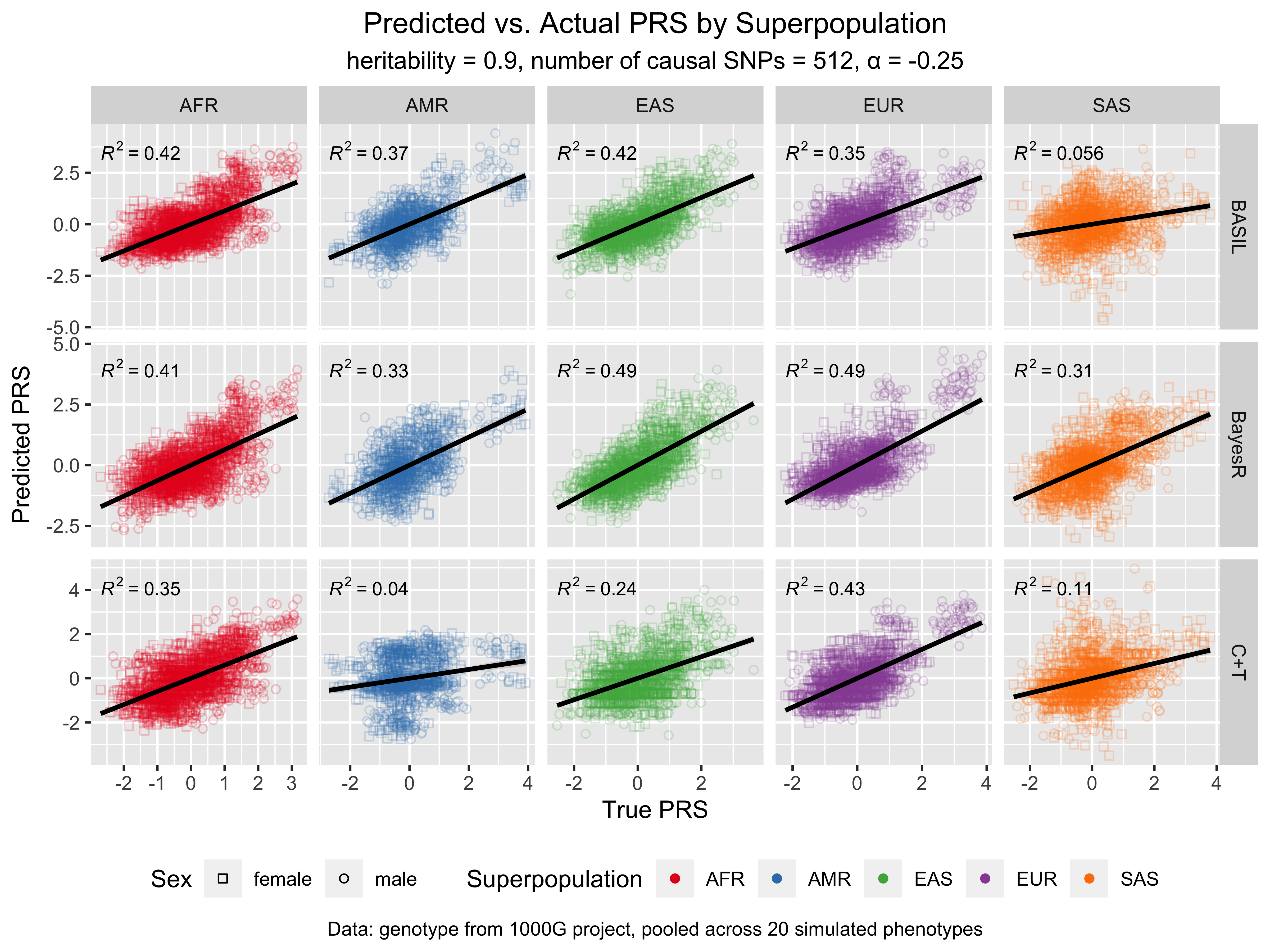
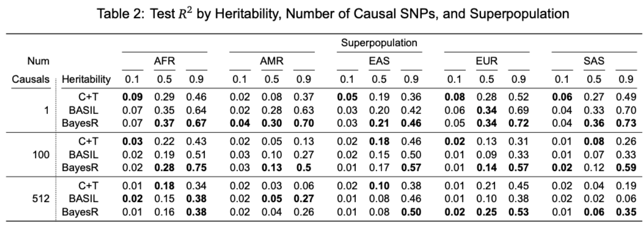
• $R^2$ (coefficient of determination) on the testing dataset in the context of GWAS and PRS provides a measure of how well a polygenic risk score can predict (true) phenotypes.

As a proof of concept and testing of data/input requirements for different software packages, we use/transform data from PS4:

• Genotype CEU_chr19_normed.{vcf,bed,pgen} is used as training set
• Genotype GBR_chr19_normed.{vcf,bed,pgen} is used as test set
• Phenotype kgvcf_ldl.{phen,pgeno} is used as ground truth phenotype

Table above reports the training and test set performance across the three methods. All three methods overfit on their own dataset. C+T and BASIL achieve similar performance on test set, while BayesR performs much better on the test set.

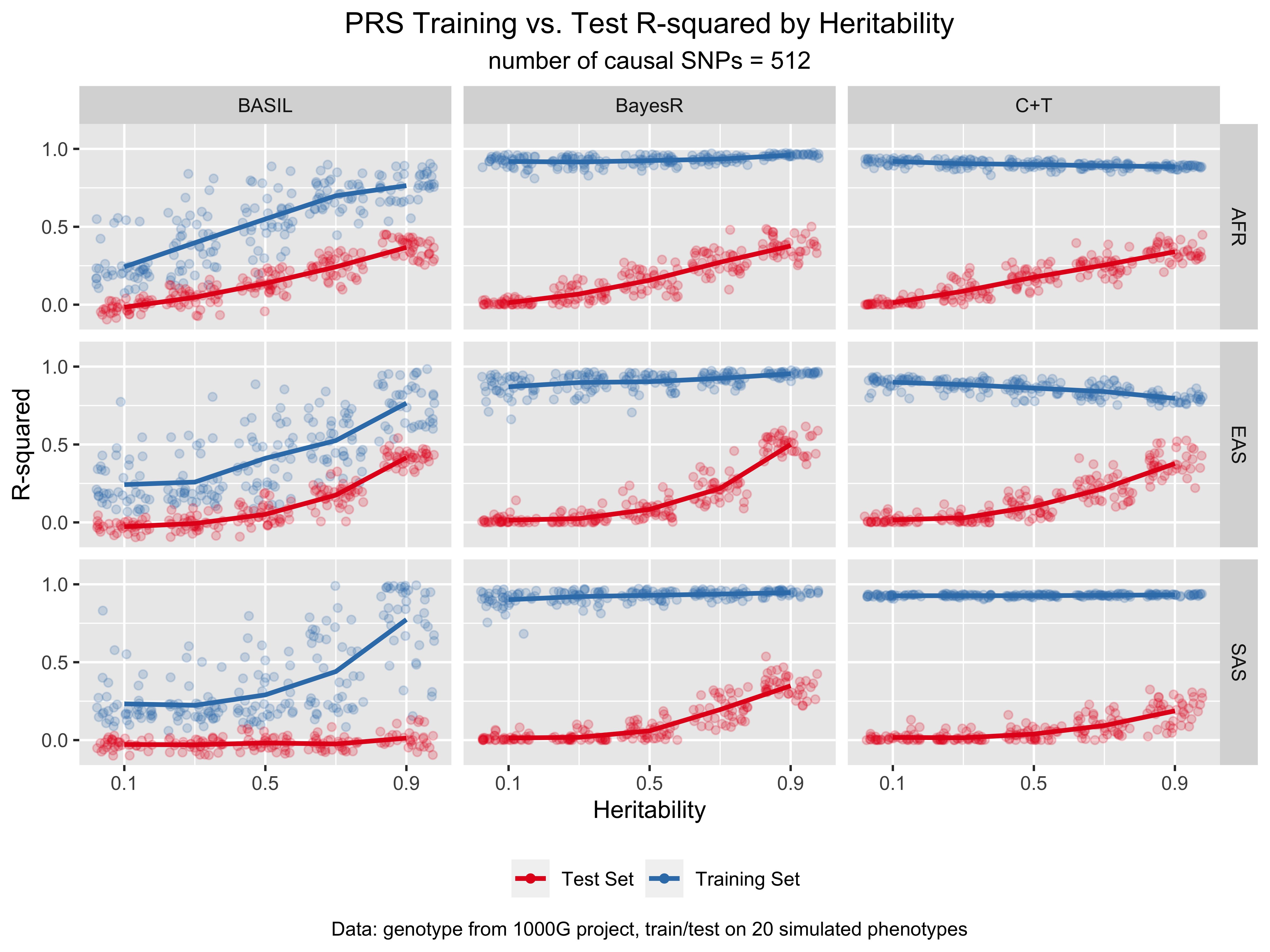
For more results and the code for replicating the figures, see notebook/42_chr19_prs_by_superpopulation_analysis.Rmd

• PLINK 1.9 and PLINK 2.0 have different input formats and modifiers. This makes data preparation and preprocessing taking a huge chunk of time. In this project, we prioritize using PLINK 2.0 since PLINK 2.0 runs faster than PLINK 1.9 in most cases, and only switch to PLINK 1.9 when PLINK 2.0 fails to accomplish what we expect or require significant modifications.
• The number of samples of each superpopulation from 1000 Genomes Project vary a lot. Therefore, the comparison results across superpopulations may not be representative.

• Different distributions of effect sizes and causal SNPs from different traits.

• Frank Dudbridge (2013) provided a comprehensive overview of the power and predictive accuracy of PRS, highlighting the statistical principles underpinning these methods and their implications for disease risk prediction.
• The 1000 Genomes Project Consortium (2015) provided a landmark achievement in human genetics, offering a global reference for human genetic variation. This comprehensive dataset has been instrumental in PRS research, allowing for the assessment of methodological performance across diverse genetic backgrounds.
• Vilhjálmsson et al. (2015) introduced a significant advancement with LDPred, a Bayesian method considering linkage disequilibrium and polygenic traits. This approach marked a step forward in PRS accuracy, emphasizing the complexity of genetic architecture in disease prediction.
• Khera et al. (2018) showcased the practical application of PRS, particularly in predicting coronary artery disease, underscoring the importance of large reference datasets for improving prediction accuracy. Their work emphasized the clinical utility of PRS, driving further research into methodological improvements.
• Lloyd-Jones et al. (2019) refined the Bayesian approach to PRS with BayesR, demonstrating the method's capability to enhance predictive power by incorporating SNP effect sizes more accurately. This study contributed to the growing preference for Bayesian models in complex disease prediction.
• Ge et al. (2019) evaluated various PRS methods, revealing performance variability across diseases and traits. Their findings stressed the necessity for flexible PRS methodologies adaptable to different genetic architectures.
• Qian et al. (2020) presented a scalable framework for Lasso-based sparse regression with BASIL in the snpnet package, efficiently handling ultra-high-dimensional genetic data. This approach represents a leap forward in managing large-scale datasets for PRS calculation.
• Yi Ding (2023) brought critical attention to the variability of polygenic scoring accuracy across different genetic ancestries. Their results highlight the need to move away from discrete genetic ancestry clusters towards the continuum of genetic ancestries when considering PGSs.

• Dudbridge F. (2013) Power and Predictive Accuracy of Polygenic Risk Scores. PLOS Genetics 9(3): e1003348. https://doi.org/10.1371/journal.pgen.1003348
• The 1000 Genomes Project Consortium. (2015) A global reference for human genetic variation. Nature 526, 68–74 https://doi.org/10.1038/nature15393
• Vilhjálmsson, B. J., Yang, J., Finucane, H. K. et al. (2015) Modeling Linkage Disequilibrium Increases Accuracy of Polygenic Risk Scores. American journal of human genetics. 97(4), 576–592. https://doi.org/10.1016/j.ajhg.2015.09.001
• Khera, A.V., Chaffin, M., Aragam, K.G. et al. (2018) Genome-wide polygenic scores for common diseases identify individuals with risk equivalent to monogenic mutations. Nat Genet 50, 1219–1224. https://doi.org/10.1038/s41588-018-0183-z
• Lloyd-Jones, L.R., Zeng, J., Sidorenko, J. et al. (2019) Improved polygenic prediction by Bayesian multiple regression on summary statistics. Nat Commun 10, 5086. https://doi.org/10.1038/s41467-019-12653-0
• Ge, T., Chen, CY., Ni, Y. et al. (2019) Polygenic prediction via Bayesian regression and continuous shrinkage priors. Nat Commun 10, 1776. https://doi.org/10.1038/s41467-019-09718-5
• Speed, D., Holmes, J. & Balding, D.J. (2020) Evaluating and improving heritability models using summary statistics. Nat Genet 52, 458–462. https://doi.org/10.1038/s41588-020-0600-y
• Qian J, Tanigawa Y, Du W, Aguirre M, Chang C, Tibshirani R, et al. (2020) A fast and scalable framework for large-scale and ultrahigh-dimensional sparse regression with application to the UK Biobank. PLoS Genet 16(10): e1009141. https://doi.org/10.1371/journal.pgen.1009141
• Ding, Y., Hou, K., Xu, Z. et al. (2023) Polygenic scoring accuracy varies across the genetic ancestry continuum. Nature 618, 774–781. https://doi.org/10.1038/s41586-023-06079-4
• UCSD CSE 284 Lecture Slides and Problem Sets