Time Series Forecasting

(with Kaggle data)

About me

Jamel Belgacem LinkedIn

R | Python | SQL | Java
I am an Application Engineer with a passion for data analysis and machine learning.

Introduction

Time series forecasting is one of the most important prediction techniques in business. The idea is to use historical data to predict future observations.

I will use the data of Store Sales-Time Series Forecasting in Kaggle competition. It is about sales in Ecuador between 2013 and 2017. You can download it from Kaggle or by cloning this repo.

I will use these libraries in this project:

library(tidymodels)
library(modeltime)
library(tseries)
library(stats)
library(zoo)
library(lubridate)
library(timetk)

Data analysis

Reading

Let's begin by reading the csv files.

df_train=read.csv(file="data/train.csv", 
                  header=TRUE, sep=",", 
                  colClasses=c("integer","Date","factor","factor","numeric","numeric"))

df_test=read.csv(file="data/test.csv", 
                 header=TRUE, sep=",",
                 colClasses=c("integer","Date","factor","factor","numeric"))

df_oil = read.csv(file="data/oil.csv", 
                  header=TRUE, sep=",",
                  colClasses=c("Date","numeric"))

df_holidays = read.csv(file="data/holidays_events.csv", 
                       header=TRUE, sep=",",
                       colClasses=c("Date","factor","factor","factor","character","factor"))

df_stores = read.csv(file="data/stores.csv",
                     header=TRUE, sep=",",
                     colClasses =c("factor","factor","factor","factor","integer"))

df_transactions = read.csv(file="data/transactions.csv", 
                           header=TRUE, sep=",",
                           colClasses=c("Date","factor","numeric"))

Summary

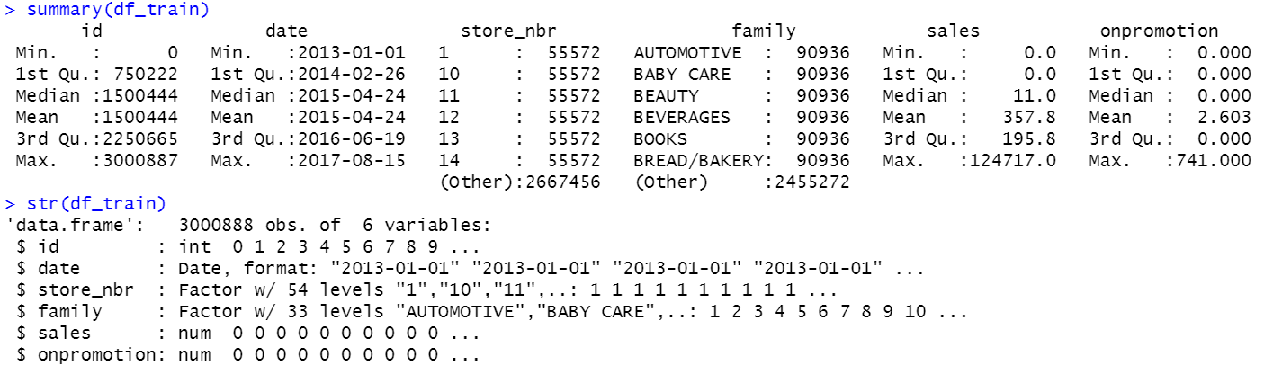
Before jumping into model creation, it is always good to take a look into our data.

summary(df_train)
str(df_train)
summary(df_oil)
str(df_oil)
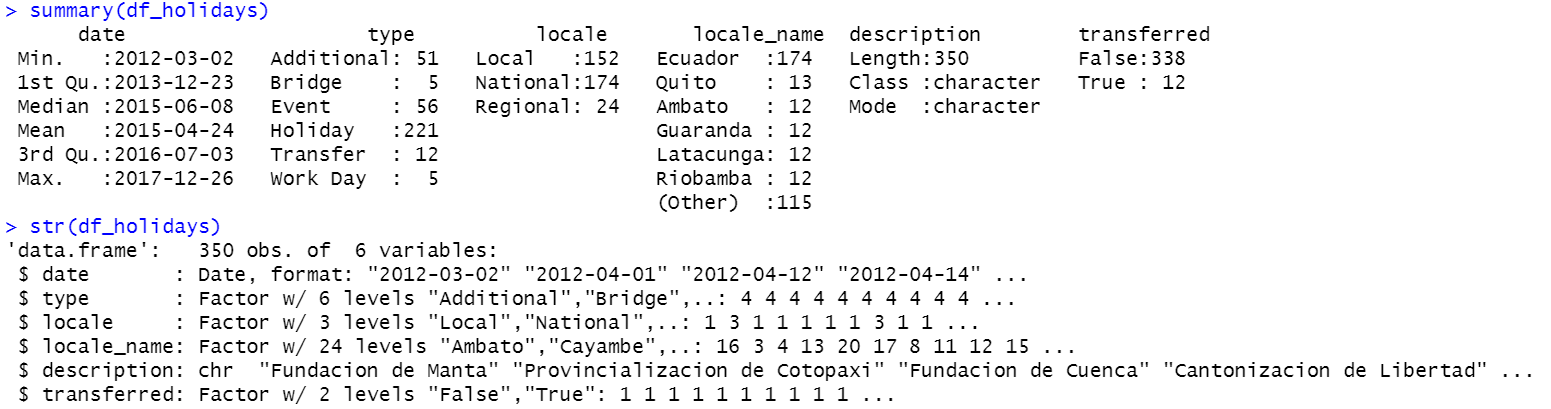
summary(df_holidays)
str(df_holidays)
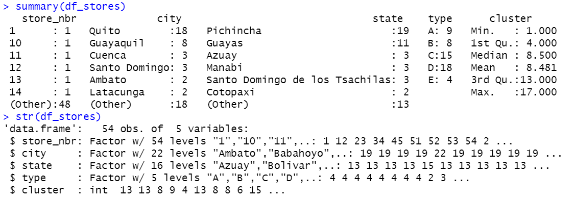
summary(df_stores)
str(df_stores)
summary(df_transactions)
str(df_transactions)

In Oil dataset's summary, you can see that it contains some missing values (NA).There is a lot of technics to deal with NA, one of them is simply delete them. In this tutorial I will take the last non NA value to replace the missing values.

df_oil$oil_NNA<-df_oil$dcoilwtico
df_oil[1,3]=df_oil[2,3]
for(i in 2:nrow(df_oil)){
  if(is.na(df_oil[i,3])){
    df_oil[i,3]=prev_val
  }else{
    prev_val=df_oil[i,3]
  }
}

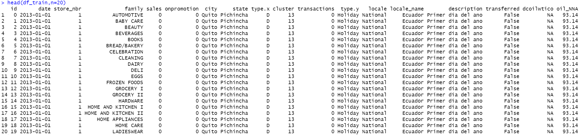
Data are separated in 6 csv files, for better understanding I will join them into one table using left join (same logic as SQL left join).

df_train <- left_join(x=df_train, y=df_stores, by="store_nbr")
df_train <- left_join(x=df_train, y=df_transactions, by=c("store_nbr","date"))
df_train <- left_join(x=df_train, y=df_holidays, by="date")
df_train <- left_join(x=df_train, y=df_oil, by="date")
head(df_train,n=20)

Analysis

Daily sales plot

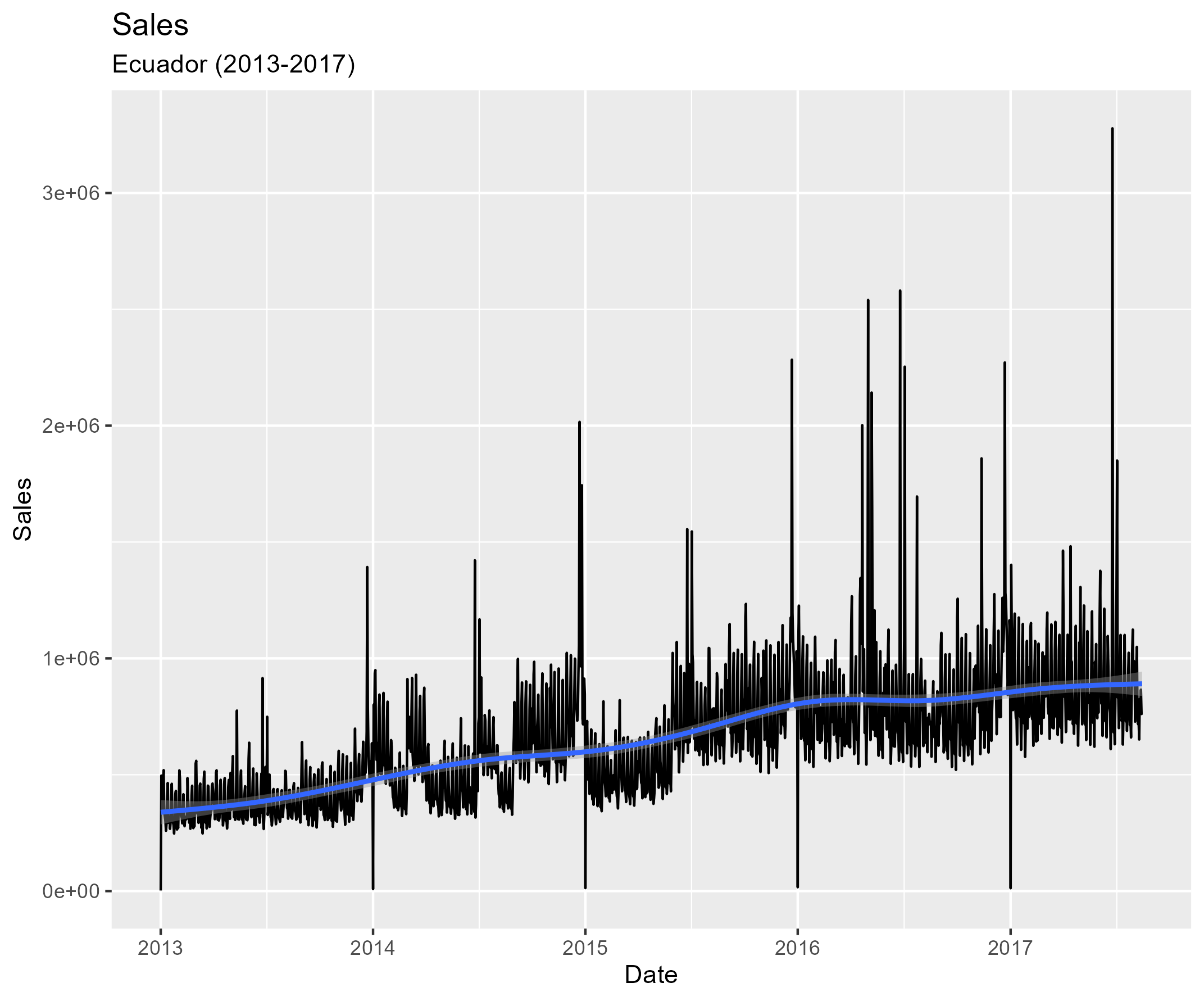
Sales in Ecuador increased between 2013 and 2017 (in 2017 almost twice as much as in 2013). We notice sales peaks in the end of each year.

plot1<-df_train %>%
  group_by(date) %>%
  summarise(
    daily_sales=sum(sales)
  ) %>%
  ggplot(aes(x=date,y=daily_sales,groups=1))+geom_line()+geom_smooth()+
  labs(title="Sales",subtitle="Ecuador (2013-2017)")+
  xlab("Date")+ylab("Sales")
ggsave("pics/plot1.png")

Oil dependency

Oil price fluctuation have a big impact on economy, and Ecuador has a high dependency on oil.

plot_salesvsoil <-df_train %>%
  group_by(date) %>%
  summarise(
    daily_sales=sum(sales,na.rm=TRUE),
    daily_oil=mean(oil_NNA,na.rm=TRUE)
  ) %>%
  ggplot(aes(x=daily_oil,y=daily_sales))+geom_point()+geom_smooth()+
  ylim(c(300000,1200000))+
  labs(title="Impact of oil price",subtitle="Ecuador (2013-2017)")+
  xlab("Oil Price")+ylab("Daily sales")
ggsave("pics/plot_oil.png")

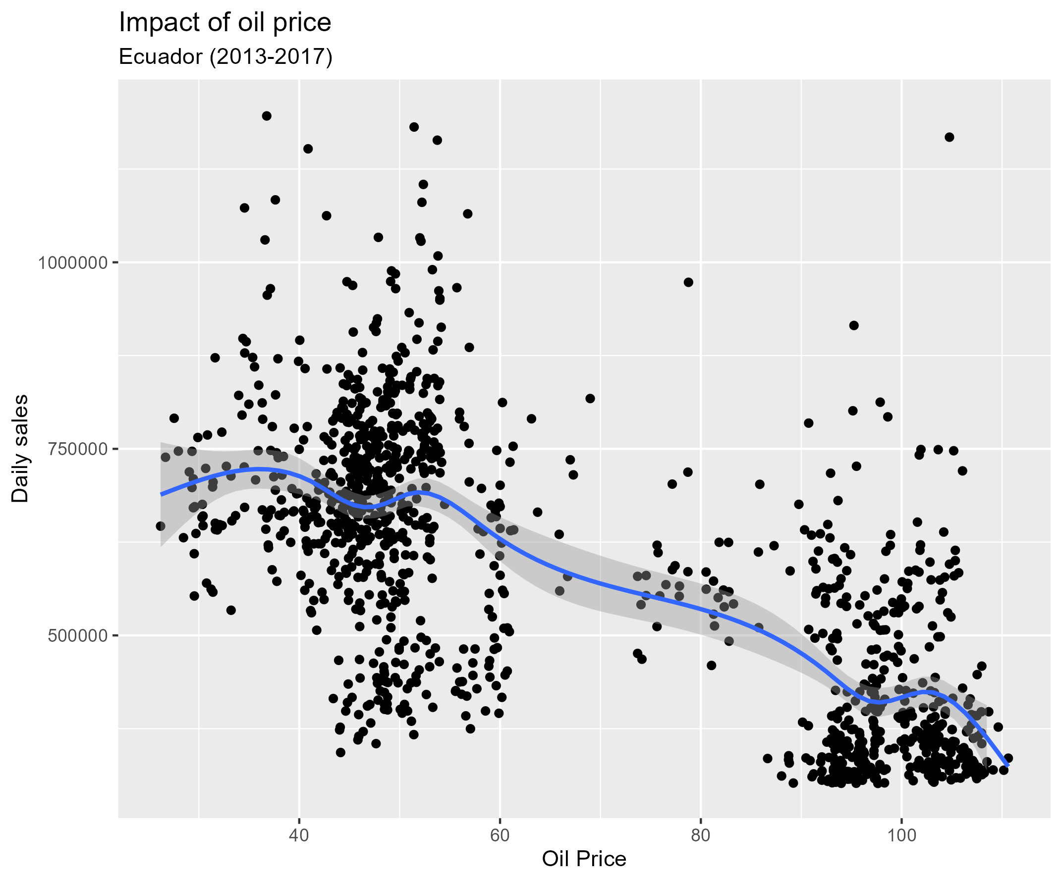
Blue line is the trend of daily sales versus oil price, sales have decreased with the increase of oil price.

Holidays/events

There are national (approx. 14), regional and local holidays in Ecuador. If we focus on national holidays, we can see that the sales volume is more important during holidays.

plot_holidays <-df_train %>%
  mutate(holidays_fact=ifelse(is.na(locale) | locale!="National","No","Yes")) %>%
  group_by(date) %>%
  summarise(
    daily_sales=sum(sales,na.rm=TRUE),
    holidays_fact=min(holidays_fact,na.rm=TRUE)
  )%>%
  mutate(holidays_fact=factor(holidays_fact,levels=c("No","Yes"))) %>%
  ggplot(aes(x=holidays_fact,y=daily_sales,fill=holidays_fact,group=holidays_fact))+geom_boxplot()+
  labs(title="Average sales",subtitle="Ecuador (2013-2017)")+xlab("Holidays ?")+ylab("Average daily sales")
ggsave("pics/plot_holidays.png")

Promotions

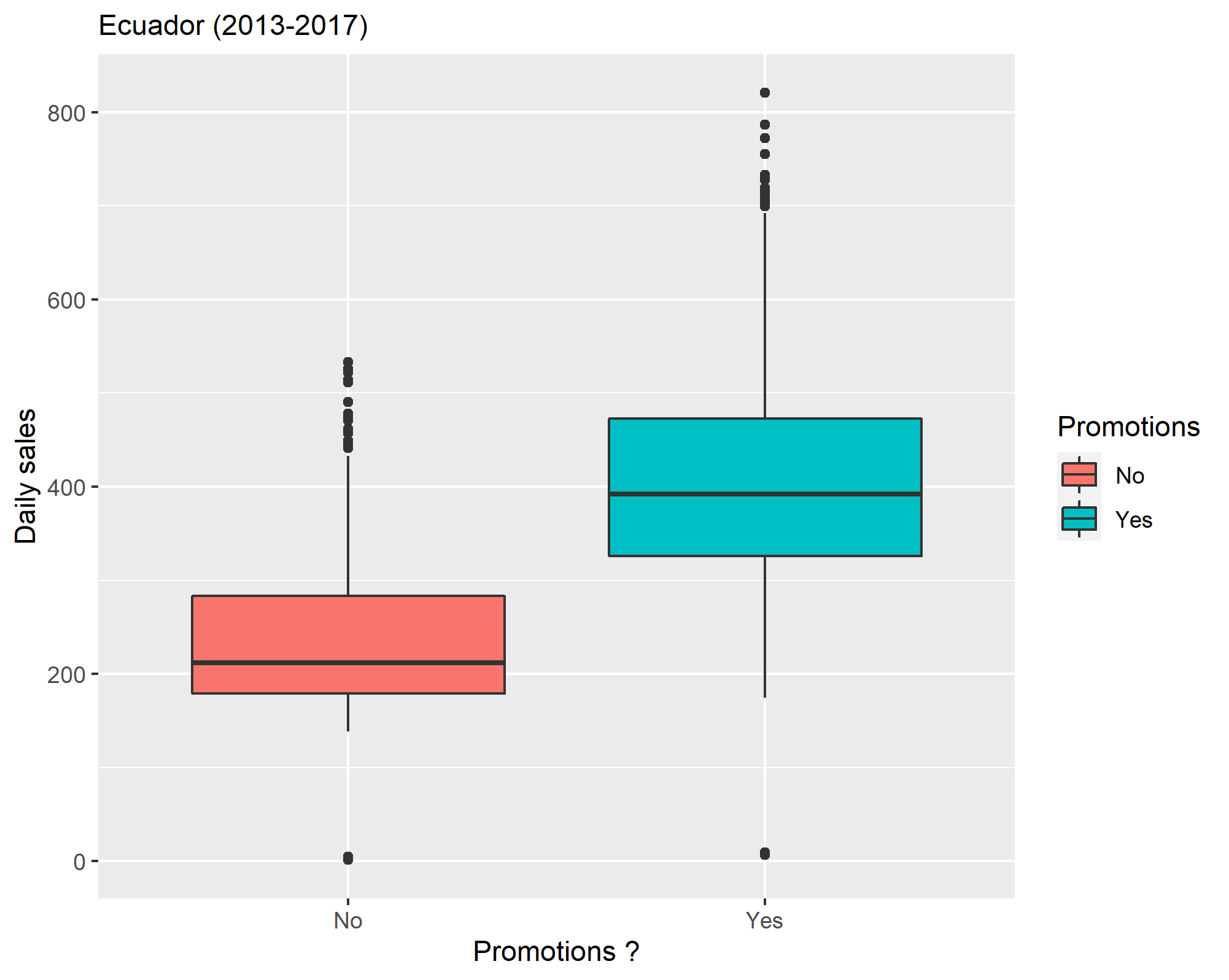
Sales promotions can have a positive effect on business, we can see it in the next plot that sales volume was more significant during promotions.

# Promotions
Plot_promotions <- df_train %>%
  group_by(date) %>%
  summarise(
    sales=mean(sales,na.rm=TRUE),
    onprom=sum(onpromotion,na.rm=TRUE)
  ) %>%
  mutate(Promotions=ifelse(onprom==0,"No","Yes")) %>%
  ggplot(aes(x=Promotions,y=sales,fill=Promotions))+geom_boxplot()+
  labs("Influence of promotions on daily sales",subtitle="Ecuador (2013-2017)")+
  xlab("Promotions ?")+ylab("Daily sales")
ggsave("pics/plot_promotions.png")

Stationarity

Stationarity is a very important aspect as our data involves time, it is important that the bahavior of our data (mean, variance) remains constant to predict the futur. We have to look into the sales variation in time to see any frequency.
To do that, we can use stl function (Seasonal Decomposition of Time Series by Loess).

# Seasonal decomposition
max_date=max(df_train$date)
min_date=min(df_train$date)

dat_ts <- df_train %>%
  # Earth quake filter
  filter(!grepl("Terremoto", description, fixed = TRUE)) %>%
  
  select(date,sales) %>%
  group_by(date) %>%
  summarise(
    value=sum(sales,na.rm=TRUE)
  )

dat_ts <-ts(dat_ts$value,end=c(year(max_date), month(max_date)),
            start=c(year(min_date), month(min_date)),
            frequency = 30)

# Seasonal Decomposition Plot
png(file="pics/stl_plot.png",
    width = 960, height = 960, units = "px", pointsize = 20,
    bg="azure")
plot(stl(dat_ts,s.window = "periodic"), 
     main="Seasonal Decomposition of Time Series by Loess")
dev.off()

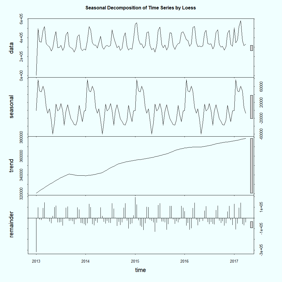
Our data shows some seasonality, we can decompose it into sum of three elements:
- Seasonal component: yearly as shown on the plot, we can add holidays and promotions in this component
- Trend component: can be explained by oil price decreasing
- Remainder component: residuals form seasonal and trend components

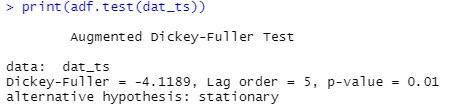
Also, We can use the Dickey-Fuller test to check the stationarity.

# Augmented Dickey-Fuller(ADF) Test
# p-value <0.05 -> data is "stationary"
print(adf.test(dat_ts))

We can affirm that our data is stationary, we can move to the next level which is forecasting.

Forecasting

There is a lot of time series forecasting models, we can sort them into three categories:

Automatic models: are the simplest and the easiest to implement.
Machine learning models: are more complex and the process much more customized,
Boosted models: using XGBoost(Extreme Gradient Boosting)

I will focus on the store number 51:

# Store_nbr 51
data<- df_train %>%
  filter(!grepl("Terremoto", description, fixed = TRUE)) %>%
  filter(store_nbr==51) %>%
  group_by(date) %>%
  summarise(
    value=mean(sales,na.rm=TRUE)
  )

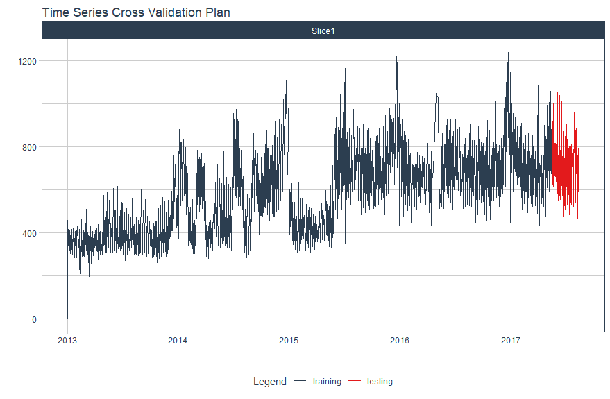
Next step, I will split my data in two using time_series_split:

training(splits) (training set)
testing(splits) (last three months as testing set)

splits <- data %>%
  time_series_split(assess = "3 months", cumulative = TRUE)

splits %>%
  tk_time_series_cv_plan() %>%
  plot_time_series_cv_plan(date, value, .interactive = FALSE)

Automatic models

ARIMA

ARIMA is abbreviation of Auto Regressive Integrative Moving Average. It is a combination of a moving average and autoregressive model. The only mode possible is regression, for engine you have two possibilities:

auto_arima: for rapid estimation of model (by default)
arima: where you can adapt manually the settings of model

model_fit_arima <- arima_reg() %>%
  set_engine("auto_arima") %>%
  fit(value ~ date, training(splits))

Prophet

Prophet is open-source software developed by Meta and available on R and Python. It is a additive technique that combines trend component, seasonality, holidays and residuals.

model_fit_prophet <- prophet_reg(seasonality_yearly = TRUE,seasonality_weekly =TRUE) %>%
  set_engine("prophet",holidays=df_holidays) %>%
  fit(value ~ date, training(splits))

TBATS

TBATS is an abbreviation of Trigonometric seasonality, Box-Cox transformation, ARMA errors, Trend and Seasonal components. This model offers the possibility to deal with multiple seasonality.

model_fit_tbats<-seasonal_reg(mode="regression",
                              seasonal_period_1= "auto",
                              seasonal_period_2= "1 year",
                              seasonal_period_3= "1 month") %>%
  set_engine("tbats") %>%
  fit(value ~ date, training(splits))

Seasonal Naive

Naive method set all forecasts to the value of previous observations, Seasonal Naive methos add seasonal factor.

model_snaive <- naive_reg() %>%
  set_engine("snaive") %>%
  fit(value ~ date, training(splits))

Machine learning models

With machine learning model, we create a recipe.
Recipe is a description of the steps to be applied to our data in order to prepare it for analysis.

recipe <- recipe(value ~ date, training(splits)) %>%
  step_timeseries_signature(date) %>%
  step_fourier(date, period = c(365, 91.25, 30.42), K = 5) %>%
  step_dummy(all_nominal(),all_predictors())
recipe %>% 
  prep() %>%
  juice()

Elastic Net

In this model, we'll fit a generalized linear model with elastic net regularization.

library(glmnet)
engine_glmnet <- linear_reg(penalty = 0.01, mixture = 0.5) %>%
  set_engine("glmnet")

model_glmnet <- workflow() %>%
  add_model(engine_glmnet) %>%
  add_recipe(recipe %>% step_rm(date)) %>%
  fit(training(splits))

Random forest

Random forest is a supervised learning algorithm for regression and classification. Random Forest operates by constructing several decision trees and outputting the mean of the classes as the prediction of all the trees.

engine_rf <- rand_forest(mode="regression",trees = 50, min_n = 5) %>%
  set_engine("randomForest")

model_rf <- workflow() %>%
  add_model(engine_rf) %>%
  add_recipe(recipe %>% step_rm(date)) %>%
  fit(training(splits))

Prophet with boost

Now, let's try the prophet model but this time with xgboost (extreme gradient boosting).

engine_prophet_boost <- prophet_boost() %>%
  set_engine("prophet_xgboost") 
workflow_fit_prophet_boost <- workflow() %>%
  add_model(model_spec_prophet_boost) %>%
  add_recipe(recipe_spec) %>%
  fit(training(splits))

Results

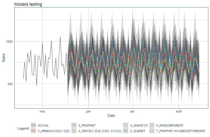
Now it's time to test all this models on test data. To compare all the models, we can regroup them into one table using modeltime_table function.

models_table <- modeltime_table(
  model_arima,
  model_prophet,
  model_tbats,
  model_snaive,
  model_glmnet,
  model_rf,
  model_prophet_boost
) 


calib_table <- models_table %>%
  modeltime_calibrate(testing(splits))

calib_table %>%
  modeltime_accuracy() %>%
  arrange(desc(rsq)) %>%
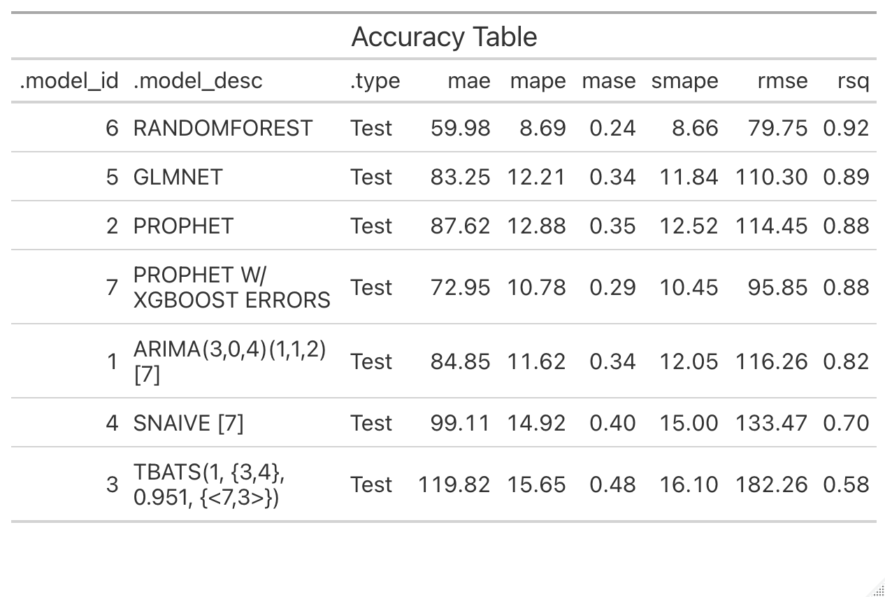
  table_modeltime_accuracy(.interactive = FALSE)

All products

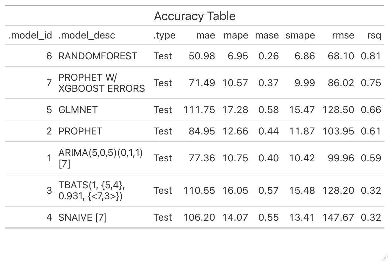
Definition of columns:

MAE: Mean absolute error
MAPE: Mean absolute percentage error
MASE: Mean absolute scaled error
SMAPE: Symmetric mean absolute percentage error
RMSE: Root mean squared error
RSQ: R-squared

The table is in descending order by RSQ. We can see that:

Random forest model is the best model with 81%
Boosted prophet offer a better RSQ than prophet

Once the model is chosen, we can apply it to make prediction on new data. This is similar to making prediction on test dataset to evaluate the model except that we need to refit our model this time using all the dataset (training+testing). You can change the period of forecast via the parameter h (3 months in this tutorial).

# 3 months prediction
## All products
calib_table %>%
  # Take Random forest model
  filter(.model_id == 6) %>%
  # Refit
  modeltime_refit(data) %>%
  modeltime_forecast(h = "3 month", actual_data = tail(data,600)) %>%
  plot_modeltime_forecast(.y_lab="Sales",.x_lab="Date",
                          .title="Sales forecasting-Sales_nbr 51-All products",
                          .interactive = FALSE,.smooth=FALSE)

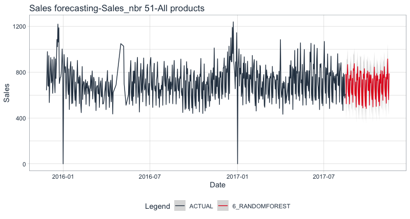
RSQ is relatively good, keep in mind that it is sales forecasting for all the products in store 51.
To see all the products for sale in the store:

df_train %>%
  filter(store_nbr==51) %>%
  distinct(family)

Now let's see the forecasting for some products.

Product 1: MEATS

Product 2: PRODUCE

Product 3: BEVERAGES

Summary

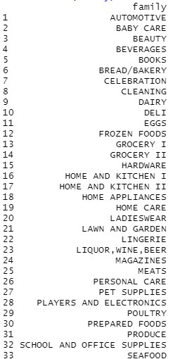
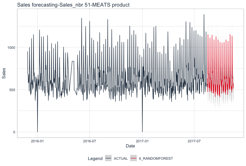
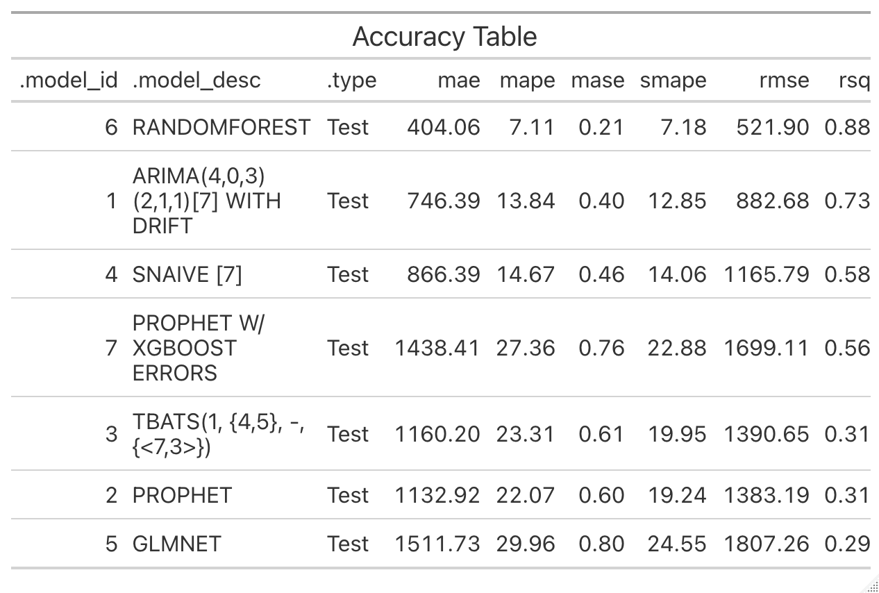
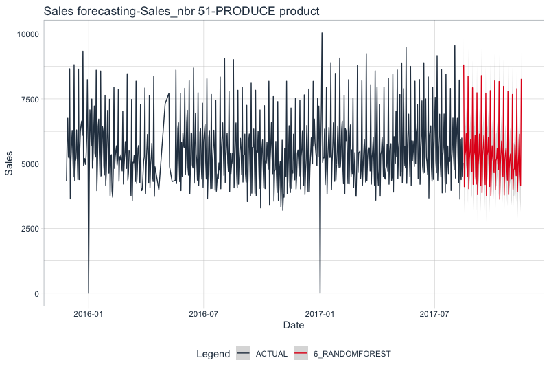
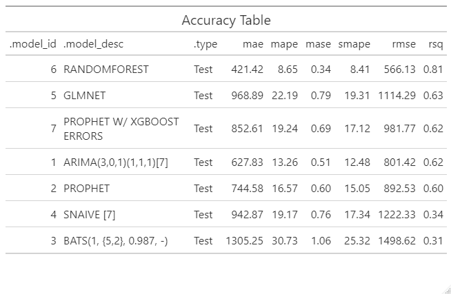
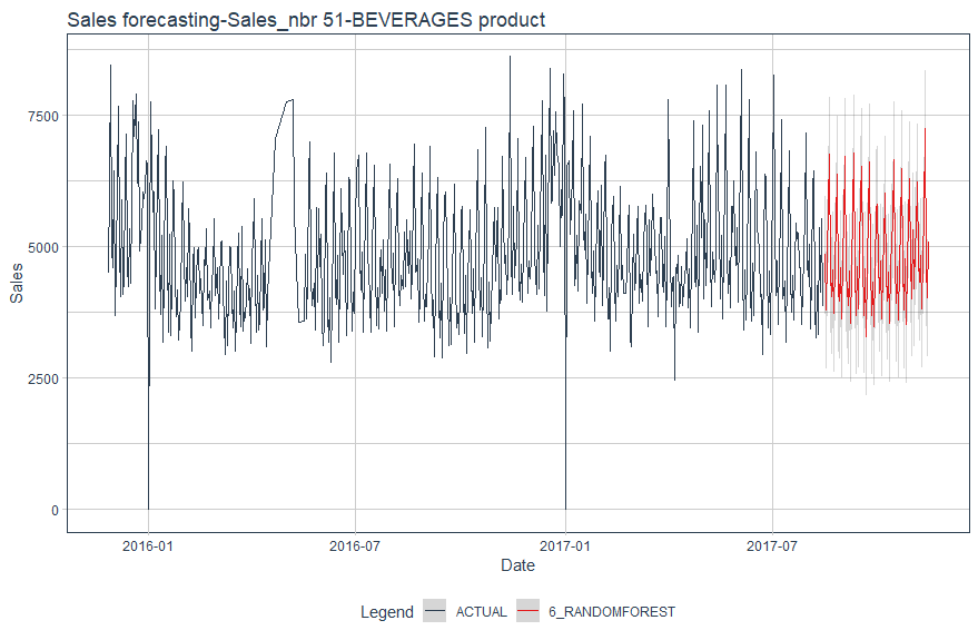
We have a better results if we forecast product by product.
For the three previous products, Random Forest model is confirmed as the best forecasting model.

jambelg / time-series-forecasting-with-r Goto Github PK