For binary classification. everybody loves the Area Under the Curve (AUC) metric, but nobody directly targets it in their loss function. Instead folks use a proxy function like Binary Cross Entropy (BCE).
This works fairly well, most of the time. But we're left with a nagging question : could we get a higher score with a loss function closer in nature to AUC?
It seems likely since BCE really bears very little relation to AUC. There have been many attempts to find a loss function that more directly targets AUC. (One common tactic is some form of rank-loss function such as Hinge Rank-Loss.) In practice, however, no clear winner has ever emerged. There's been no serious challenge to BCE.
There are also considerations beyond performance. Since BCE is essentially different than AUC, BCE tends to misbehave in the final stretch of training where we are trying to steer it toward the highest AUC score.
A good deal of the AUC optimization actually ends up occurring in the tuning of hyper-parameters. Early Stopping becomes an uncomfortable necessity as the model may diverge sharply at any time from its high score.
We'd like a loss function that gives us higher scores and less trouble.
We present such a function here.
My favorite working definition of AUC is this: Let's call the binary class labels "Black" (0) and "White" (1). Pick one black element at random and let x be its predicted value. Now pick a random white element with value y. Then,
AUC = the probability that the elements are in the right order. That is, x<y .
That's it. For any given set of points like the Training Set, we can get this probability by doing a brute-force calculation. Scan the set of all possible black/white pairs , and count the portion that are right-ordered.
We can see that the AUC score is not differentiable (a smooth curve with respect to any single x or y.) Take an element (any color) and move it slightly enough that it doesn't hit a neighboring element. The AUC stays the same. Once the point does cross a neighbor, we have a chance of flipping one of the x<y comparisons - which changes the AUC. So the AUC makes no smooth transitions.
That's a problem for Neural Nets, where we need a differentiable loss function.
So we set out to find a differentiable function which is close as possible to AUC.
I dug back through the existing literature and found nothing that worked in practice. Finally I came across a curious piece of code that somebody had checked into the TFLearn codebase.
Without fanfare, it promised differentiable deliverance from BCE in the form of a new loss function.
(Don't try it, it blows up.) : http://tflearn.org/objectives/#roc-auc-score
def roc_auc_score(y_pred, y_true):
"""Bad code, do not use.
ROC AUC Score.
Approximates the Area Under Curve score, using approximation based on
the Wilcoxon-Mann-Whitney U statistic.
Yan, L., Dodier, R., Mozer, M. C., & Wolniewicz, R. (2003).
Optimizing Classifier Performance via an Approximation to the Wilcoxon-Mann-Whitney Statistic.
Measures overall performance for a full range of threshold levels.
Arguments:
    y_pred: `Tensor`. Predicted values.
    y_true: `Tensor` . Targets (labels), a probability distribution.
"""
with tf.name_scope("RocAucScore"):
    pos = tf.boolean_mask(y_pred, tf.cast(y_true, tf.bool))
    neg = tf.boolean_mask(y_pred, ~tf.cast(y_true, tf.bool))
 .
 .
 more bad code)
It doesn't work at all. (Blowing up is actually the least of its problems). But it mentions the paper it was based on.
Even though the paper is ancient, dating back to 2003, I found that with a little work - some extension of the math and careful coding - it actually works. It's uber-fast, with speed comparable to BCE (and just as vectorizable for a GPU/MPP) *. In my tests, it gives higher AUC scores than BCE, is less sensitive to Learning Rate (avoiding the need for a Scheduler in my tests), and eliminates entirely the need for Early Stopping.
OK, let's turn to the original paper : Optimizing Classifier Performance via an Approximation to the Wilcoxon-Mann-Whitney Statistic.
The authors, Yan et. al , motivate the discussion by writing the AUC score in a particular form. Recall our example where we calculate AUC by doing a brute-force count over the set of possible black/white pairs to find the portion that are right-ordered. Let B be the set of black values and W the set of white values. All possible pairs are given by the Cartesian Product B X W. To count the right-ordered pairs we write :
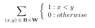
This is really just straining mathematical notation to say 'count the right-ordered pairs.' If we divide this sum by the total number of pairs , |B| * |W|, we get exactly the AUC metric. (Historically, this is called the normalized Wilcoxon-Mann-Whitney (WMW) statistic.)
To make a loss function from this, we could just flip the x < y comparison to x > y in order to penalize wrong-ordered pairs. The problem, of course, is that discontinuous jump when x crosses y .
Yan et. al surveys - and then rejects - past work-arounds using continuous approximations to the step (Heaviside) function, such as a Sigmoid curve. Then they pull this out of a hat :
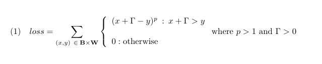
Yann got this forumula by applying a series of changes to the WMW:
- x<y has been flipped to y<x, to make it a loss (higher is worse.) So the loss is focussed on wrong-ordered pairs.
- Instead of treating all pairs equally, weight is given to the how far apart the pair is.
- That weight is raised to the power of p.
- We add a padding Γ to that distance.
We'll go through these in turn. 1 is clear enough. There's a little more to 2 than meets the eye. It makes intuitive sense that wrong-ordered pairs with wide separation should be given a bigger loss. But something interesting is also happening as that separation approaches 0. The loss goes to zero linearly, rather than a step-function. So we've gotten rid of the discontinuity.
In fact, if p were 1 and Γ were 0, the loss would simply be our old friend ReLu(x-y). But in this case we notice a hiccup, which reveals the need for the exponent p. ReLu is not differentiable at 0. That's not much of a problem in ReLu's more accustomed role as an activation function, but for our purposes the singularity at 0 lands directly on the thing we are most interested most in : the points where white and black elements pass each other.
Fortunately, raising ReLu to a power fixes this. ReLu^p with p>1 is differentiable everywhere. OK, so p>1.
Now back to Γ : Γ provides a 'padding' which is enforced between two points. We penalize not only wrong-ordered pairs, but also right-ordered pairs which are too close. If a right-ordered pair is too close, its elements are at risk of getting swapped in the future by the random jiggling of a stochastic neural net. The idea is to keep them moving apart until they reach a comfortable distance.
And that's the basic idea as outlined in the paper. We now ake some refinements regarding Γ and p.
Here we break a bit with the paper. Yan et. al seem a little squeamish on the topic of choosing Γ and p, offering only that a p = 2 or p = 3 seems good and that Γ should be somewhere between 0.10 and 0.70. Yan essentially wishes us luck with these parameters and bows out.
First, we permanently fix p = 2, because any self-respecting loss function should be a sum-of-squares. (One reason for this is that it ensures the loss function is not only differentiable, but also convex)
Second and more importantly, let's take a look at Γ. The heuristic of 'somewhere from 0.10 to 0.70' looks strange on the face of it; even if the predictions were normalized to be 0<x<1, this guidance seems overbroad, indifferent to the underlying distributions, and just weird.
We're going to derive Γ from the training set.
Consider the training set and its Black/White pairs, B X W. There are |B||W| pairs in this set. Of these, |B| |W| AUC are right-ordered. So, the number of wrong-ordered pairs is (1-AUC) |B| |W|
When Γ is zero, only these wrong-ordered pairs are in motion (have positive loss.) A positive Γ would expand the set of moving pairs to include some pairs which are right-ordered, but too close. Instead of worrying about Γ's numeric value, we'll specify just how many too-close pairs we want to set in motion:
We define a constant δ which fixes the proportion of too-close pairs to wrong-ordered pairs.
- |too_close_pairs| = δ |wrong_ordered_pairs|
We fix this δ throughout training and update Γ to conform to it. For given δ, we find Γ such that
- |pairs where y+Γ>x| = δ |pairs where y>x|
In our experiments we found that δ can range from 0.5 to 2.0, and 1.0 is a good default choice.
So we set δ to 1, p to 2, and forget about Γ altogether,
Our loss function (1) looks dismally expensive to compute. It requires that we scan the entire training set for each individual prediction.
We bypass this problem with a performance tweak :
Suppose we are calculating the loss function for a given white data point, x. To calculate (3), we need to compare x against the entire training set of black predictions, y. We take a short-cut and use a random sub-sample of the black data points. If we set the size of the sub-sample to be, say, 1000 - we get a very (very) close approximation to the true loss function. [1]
Similar reasoning applies to the loss function of a black data-point; we use a random sub-sample of all white training elements.
In this way, white and black subsamples fit easily into GPU memory. By reusing the same sub-sample throughout a given batch, we can parallelize the operation in batches. We end up with a loss function that's about as fast at BCE.
Here's the batch-loss function in PyTorch:
def roc_star_loss( _y_true, y_pred, gamma, _epoch_true, epoch_pred):
    """
    Nearly direct loss function for AUC.
    See article,
    C. Reiss, "Roc-star : An objective function for ROC-AUC that actually works."
    https://github.com/iridiumblue/articles/blob/master/roc_star.md
        _y_true: `Tensor`. Targets (labels).  Float either 0.0 or 1.0 .
        y_pred: `Tensor` . Predictions.
        gamma  : `Float` Gamma, as derived from last epoch.
        _epoch_true: `Tensor`.  Targets (labels) from last epoch.
        epoch_pred : `Tensor`.  Predicions from last epoch.
    """
    #convert labels to boolean
    y_true = (_y_true>=0.50)
    epoch_true = (_epoch_true>=0.50)

    # if batch is either all true or false return small random stub value.
    if torch.sum(y_true)==0 or torch.sum(y_true) == y_true.shape[0]: return torch.sum(y_pred)*1e-8

    pos = y_pred[y_true]
    neg = y_pred[~y_true]

    epoch_pos = epoch_pred[epoch_true]
    epoch_neg = epoch_pred[~epoch_true]

    # Take random subsamples of the training set, both positive and negative.
    max_pos = 1000 # Max number of positive training samples
    max_neg = 1000 # Max number of positive training samples
    cap_pos = epoch_pos.shape[0]
    cap_neg = epoch_neg.shape[0]
    epoch_pos = epoch_pos[torch.rand_like(epoch_pos) < max_pos/cap_pos]
    epoch_neg = epoch_neg[torch.rand_like(epoch_neg) < max_neg/cap_pos]

    ln_pos = pos.shape[0]
    ln_neg = neg.shape[0]

    # sum positive batch elements agaionst (subsampled) negative elements
    if ln_pos>0 :
        pos_expand = pos.view(-1,1).expand(-1,epoch_neg.shape[0]).reshape(-1)
        neg_expand = epoch_neg.repeat(ln_pos)

        diff2 = neg_expand - pos_expand + gamma
        l2 = diff2[diff2>0]
        m2 = l2 * l2
        len2 = l2.shape[0]
    else:
        m2 = torch.tensor([0], dtype=torch.float).cuda()
        len2 = 0

    # Similarly, compare negative batch elements against (subsampled) positive elements
    if ln_neg>0 :
        pos_expand = epoch_pos.view(-1,1).expand(-1, ln_neg).reshape(-1)
        neg_expand = neg.repeat(epoch_pos.shape[0])

        diff3 = neg_expand - pos_expand + gamma
        l3 = diff3[diff3>0]
        m3 = l3*l3
        len3 = l3.shape[0]
    else:
        m3 = torch.tensor([0], dtype=torch.float).cuda()
        len3=0

    if (torch.sum(m2)+torch.sum(m3))!=0 :
       res2 = torch.sum(m2)/max_pos+torch.sum(m3)/max_neg
       #code.interact(local=dict(globals(), **locals()))
    else:
       res2 = torch.sum(m2)+torch.sum(m3)

    res2 = torch.where(torch.isnan(res2), torch.zeros_like(res2), res2)

    return res2
Note that there are some extra parameters. We are passing in the training set from the last epoch. Since the entire training set doesn't change much from one epoch to the next, the loss function can compare each prediction again a slightly out-of-date training set. This simplifies debugging, and appears to benefit performance as the 'background' epoch isn't changing from one batch to the next.
Similarly, Γ is an expensive calculation. We again use the sub-sampling trick, but increase the size of the sub-samples to ~10,000 to ensure an accurate estimate. To keep performance clipping along, we recompute this value only once per epoch. Here's the function to do that :
def epoch_update_gamma(y_true,y_pred, epoch=-1,delta=2):
    """
    Calculate gamma from last epoch's targets and predictions.
    Gamma is updated at the end of each epoch.
    y_true: `Tensor`. Targets (labels).  Float either 0.0 or 1.0 .
    y_pred: `Tensor` . Predictions.
    """
    DELTA = delta
    SUB_SAMPLE_SIZE = 2000.0
    pos = y_pred[y_true==1]
    neg = y_pred[y_true==0] # yo pytorch, no boolean tensors or operators?  Wassap?
    # subsample the training set for performance
    cap_pos = pos.shape[0]
    cap_neg = neg.shape[0]
    pos = pos[torch.rand_like(pos) < SUB_SAMPLE_SIZE/cap_pos]
    neg = neg[torch.rand_like(neg) < SUB_SAMPLE_SIZE/cap_neg]
    ln_pos = pos.shape[0]
    ln_neg = neg.shape[0]
    pos_expand = pos.view(-1,1).expand(-1,ln_neg).reshape(-1)
    neg_expand = neg.repeat(ln_pos)
    diff = neg_expand - pos_expand
    ln_All = diff.shape[0]
    Lp = diff[diff>0] # because we're taking positive diffs, we got pos and neg flipped.
    ln_Lp = Lp.shape[0]-1
    diff_neg = -1.0 * diff[diff<0]
    diff_neg = diff_neg.sort()[0]
    ln_neg = diff_neg.shape[0]-1
    ln_neg = max([ln_neg, 0])
    left_wing = int(ln_Lp*DELTA)
    left_wing = max([0,left_wing])
    left_wing = min([ln_neg,left_wing])
    default_gamma=torch.tensor(0.2, dtype=torch.float).cuda()
    if diff_neg.shape[0] > 0 :
       gamma = diff_neg[left_wing]
    else:
       gamma = default_gamma # default=torch.tensor(0.2, dtype=torch.float).cuda() #zoink
    L1 = diff[diff>-1.0*gamma]
    ln_L1 = L1.shape[0]
    if epoch > -1 :
        return gamma
    else :
        return default_gamma
Here's the helicopter view showing how to use the two functions as we loop on epochs, then on batches :
train_ds = CatDogDataset(train_files, transform)
train_dl = DataLoader(train_ds, batch_size=BATCH_SIZE)

#initialize last epoch with random values
last_epoch_y_pred = torch.tensor( 1.0-numpy.random.rand(len(train_ds))/2.0, dtype=torch.float).cuda()
last_epoch_y_t    = torch.tensor([o for o in train_tt],dtype=torch.float).cuda()
epoch_gamma = 0.20
for epoch in range(epoches):
    epoch_y_pred=[]
    epoch_y_t=[]
    for X, y in train_dl:
        preds = model(X)
        # .
        # .
        loss = roc_star_loss(y,preds,epoch_gamma, last_epoch_y_t, last_epoch_y_pred)
        # .
        # .
        epoch_y_pred.extend(preds)
        epoch_y_t.extend(y)
    last_epoch_y_pred = torch.tensor(epoch_y_pred).cuda()
    last_epoch_y_t = torch.tensor(epoch_y_t).cuda()
    epoch_gamma = epoch_update_gamma(last_epoch_y_t, last_epoch_y_pred, epoch)
    #...
A complete working example can be found here, example.py For a faster jump-star you can fork this kernel on Kaggle : kernel
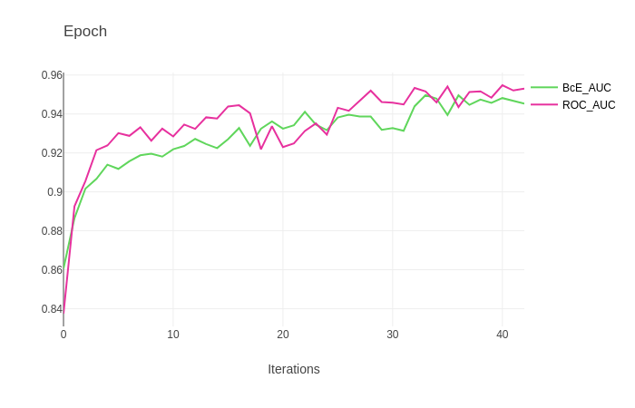
Below we chart the performance of roc-star against the same model using BCE. Experience shows that roc-star can often simply be swapped into any model using BCE with a good chance at a performance increase.