After SELECT and FROM, the next SQL clause you're most likely to use as a data scientist is WHERE.
With just a SELECT expression, we can specify which columns we want to select, as well as transform the column values using aliases, built-in functions, and other expressions.
However if we want to filter the rows that we want to select, we also need to include a WHERE clause.
You will be able to:
- Retrieve a subset of records from a table using a
WHEREclause - Filter results using conditional operators such as
BETWEEN,IS NULL, andLIKE - Apply an aggregate function to the result of a filtered query
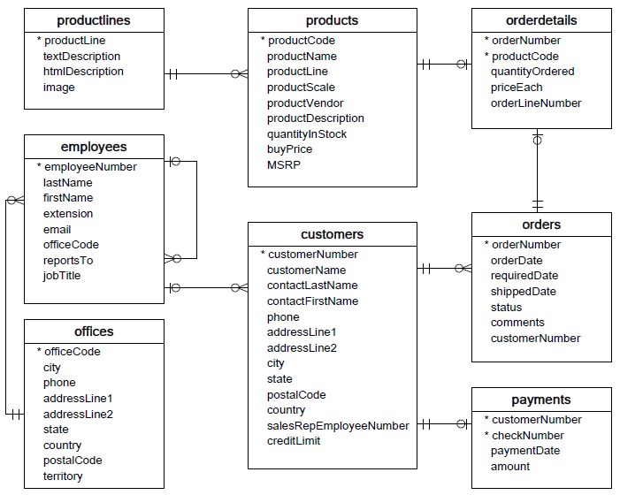
For this section of the lesson, we'll use the Northwind database, the ERD (entity-relationship diagram) of which is shown below:
Below, we connect to a SQLite database using the Python sqlite3 library (documentation here), then display the contents of the employees table:
import pandas as pd
import sqlite3
conn = sqlite3.connect('data.sqlite')
pd.read_sql("""
SELECT *
  FROM employees;
""", conn).dataframe tbody tr th {
vertical-align: top;
}
.dataframe thead th {
text-align: right;
}
| employeeNumber | lastName | firstName | extension | officeCode | reportsTo | jobTitle | ||
|---|---|---|---|---|---|---|---|---|
| 0 | 1002 | Murphy | Diane | x5800 | [email protected] | 1 | President | |
| 1 | 1056 | Patterson | Mary | x4611 | [email protected] | 1 | 1002 | VP Sales |
| 2 | 1076 | Firrelli | Jeff | x9273 | [email protected] | 1 | 1002 | VP Marketing |
| 3 | 1088 | Patterson | William | x4871 | [email protected] | 6 | 1056 | Sales Manager (APAC) |
| 4 | 1102 | Bondur | Gerard | x5408 | [email protected] | 4 | 1056 | Sale Manager (EMEA) |
| 5 | 1143 | Bow | Anthony | x5428 | [email protected] | 1 | 1056 | Sales Manager (NA) |
| 6 | 1165 | Jennings | Leslie | x3291 | [email protected] | 1 | 1143 | Sales Rep |
| 7 | 1166 | Thompson | Leslie | x4065 | [email protected] | 1 | 1143 | Sales Rep |
| 8 | 1188 | Firrelli | Julie | x2173 | [email protected] | 2 | 1143 | Sales Rep |
| 9 | 1216 | Patterson | Steve | x4334 | [email protected] | 2 | 1143 | Sales Rep |
| 10 | 1286 | Tseng | Foon Yue | x2248 | [email protected] | 3 | 1143 | Sales Rep |
| 11 | 1323 | Vanauf | George | x4102 | [email protected] | 3 | 1143 | Sales Rep |
| 12 | 1337 | Bondur | Loui | x6493 | [email protected] | 4 | 1102 | Sales Rep |
| 13 | 1370 | Hernandez | Gerard | x2028 | [email protected] | 4 | 1102 | Sales Rep |
| 14 | 1401 | Castillo | Pamela | x2759 | [email protected] | 4 | 1102 | Sales Rep |
| 15 | 1501 | Bott | Larry | x2311 | [email protected] | 7 | 1102 | Sales Rep |
| 16 | 1504 | Jones | Barry | x102 | [email protected] | 7 | 1102 | Sales Rep |
| 17 | 1611 | Fixter | Andy | x101 | [email protected] | 6 | 1088 | Sales Rep |
| 18 | 1612 | Marsh | Peter | x102 | [email protected] | 6 | 1088 | Sales Rep |
| 19 | 1619 | King | Tom | x103 | [email protected] | 6 | 1088 | Sales Rep |
| 20 | 1621 | Nishi | Mami | x101 | [email protected] | 5 | 1056 | Sales Rep |
| 21 | 1625 | Kato | Yoshimi | x102 | [email protected] | 5 | 1621 | Sales Rep |
| 22 | 1702 | Gerard | Martin | x2312 | [email protected] | 4 | 1102 | Sales Rep |
When filtering data using WHERE, you are trying to find rows that match a specific condition. The simplest condition involves checking whether a specific column contains a specific value. In SQLite, this is done using =, which is similar to == in Python:
pd.read_sql("""
SELECT *
  FROM employees
 WHERE lastName = "Patterson";
""", conn).dataframe tbody tr th {
vertical-align: top;
}
.dataframe thead th {
text-align: right;
}
| employeeNumber | lastName | firstName | extension | officeCode | reportsTo | jobTitle | ||
|---|---|---|---|---|---|---|---|---|
| 0 | 1056 | Patterson | Mary | x4611 | [email protected] | 1 | 1002 | VP Sales |
| 1 | 1088 | Patterson | William | x4871 | [email protected] | 6 | 1056 | Sales Manager (APAC) |
| 2 | 1216 | Patterson | Steve | x4334 | [email protected] | 2 | 1143 | Sales Rep |
Note that we are selecting all columns (SELECT *) but are no longer selecting all rows. Instead, we are only selecting the 3 rows where the value of lastName is "Patterson".
SQL is essentially doing something like this:
# Selecting all of the records in the database
result = pd.read_sql("SELECT * FROM employees;", conn)
# Create a list to store the records that match the query
employees_named_patterson = []
# Loop over all of the employees
for _, data in result.iterrows():
    # Check if the last name is "Patterson"
    if data["lastName"] == "Patterson":
        # Add to list
        employees_named_patterson.append(data)

# Display the result list as a DataFrame
pd.DataFrame(employees_named_patterson).dataframe tbody tr th {
vertical-align: top;
}
.dataframe thead th {
text-align: right;
}
| employeeNumber | lastName | firstName | extension | officeCode | reportsTo | jobTitle | ||
|---|---|---|---|---|---|---|---|---|
| 1 | 1056 | Patterson | Mary | x4611 | [email protected] | 1 | 1002 | VP Sales |
| 3 | 1088 | Patterson | William | x4871 | [email protected] | 6 | 1056 | Sales Manager (APAC) |
| 9 | 1216 | Patterson | Steve | x4334 | [email protected] | 2 | 1143 | Sales Rep |
Except SQL is designed specifically to perform these kinds of queries efficiently! Even if you are pulling data from SQL into Python for further analysis, SELECT * FROM <table>; is very rarely the most efficient approach. You should be thinking about how to get SQL to do the "heavy lifting" for you in terms of selecting, filtering, and transforming the raw data!
You can also combine WHERE clauses with SELECT statements other than SELECT * in order to filter rows and columns at the same time. For example:
pd.read_sql("""
SELECT firstName, lastName, email
  FROM employees
 WHERE lastName = "Patterson";
""", conn).dataframe tbody tr th {
vertical-align: top;
}
.dataframe thead th {
text-align: right;
}
| firstName | lastName | ||
|---|---|---|---|
| 0 | Mary | Patterson | [email protected] |
| 1 | William | Patterson | [email protected] |
| 2 | Steve | Patterson | [email protected] |
WHERE clauses are especially powerful when combined with more-complex SELECT statements. Most of the time you will want to use aliases (with AS) in the SELECT statements to make the WHERE clauses more concise and readable.
If we wanted to select all employees with 5 letters in their first name, that would look like this:
pd.read_sql("""
SELECT *, length(firstName) AS name_length
  FROM employees
 WHERE name_length = 5;
""", conn).dataframe tbody tr th {
vertical-align: top;
}
.dataframe thead th {
text-align: right;
}
| employeeNumber | lastName | firstName | extension | officeCode | reportsTo | jobTitle | name_length | ||
|---|---|---|---|---|---|---|---|---|---|
| 0 | 1002 | Murphy | Diane | x5800 | [email protected] | 1 | President | 5 | |
| 1 | 1188 | Firrelli | Julie | x2173 | [email protected] | 2 | 1143 | Sales Rep | 5 |
| 2 | 1216 | Patterson | Steve | x4334 | [email protected] | 2 | 1143 | Sales Rep | 5 |
| 3 | 1501 | Bott | Larry | x2311 | [email protected] | 7 | 1102 | Sales Rep | 5 |
| 4 | 1504 | Jones | Barry | x102 | [email protected] | 7 | 1102 | Sales Rep | 5 |
| 5 | 1612 | Marsh | Peter | x102 | [email protected] | 6 | 1088 | Sales Rep | 5 |
Or, to select all employees with the first initial of "L", that would look like this:
pd.read_sql("""
SELECT *, substr(firstName, 1, 1) AS first_initial
  FROM employees
 WHERE first_initial = "L";
""", conn).dataframe tbody tr th {
vertical-align: top;
}
.dataframe thead th {
text-align: right;
}
| employeeNumber | lastName | firstName | extension | officeCode | reportsTo | jobTitle | first_initial | ||
|---|---|---|---|---|---|---|---|---|---|
| 0 | 1165 | Jennings | Leslie | x3291 | [email protected] | 1 | 1143 | Sales Rep | L |
| 1 | 1166 | Thompson | Leslie | x4065 | [email protected] | 1 | 1143 | Sales Rep | L |
| 2 | 1337 | Bondur | Loui | x6493 | [email protected] | 4 | 1102 | Sales Rep | L |
| 3 | 1501 | Bott | Larry | x2311 | [email protected] | 7 | 1102 | Sales Rep | L |
Important note: Just like in Python, you can compare numbers in SQL just by typing the number (e.g. name_length = 5) but if you want to compare to a string value, you need to surround the value with quotes (e.g. first_initial = "L"). If you forget the quotes, you will get an error, because SQL will interpret it as a variable name rather than a hard-coded value:
pd.read_sql("""
SELECT *, substr(firstName, 1, 1) AS first_initial
  FROM employees
 WHERE first_initial = L;
""", conn)
---------------------------------------------------------------------------
OperationalError Traceback (most recent call last)
~/opt/anaconda3/envs/learn-env/lib/python3.8/site-packages/pandas/io/sql.py in execute(self, *args, **kwargs)
2017 try:
-> 2018 cur.execute(*args, **kwargs)
2019 return cur
OperationalError: no such column: L
The above exception was the direct cause of the following exception:
DatabaseError Traceback (most recent call last)
<ipython-input-7-083650d31057> in <module>
----> 1 pd.read_sql("""
2 SELECT *, substr(firstName, 1, 1) AS first_initial
3 FROM employees
4 WHERE first_initial = L;
5 """, conn)
~/opt/anaconda3/envs/learn-env/lib/python3.8/site-packages/pandas/io/sql.py in read_sql(sql, con, index_col, coerce_float, params, parse_dates, columns, chunksize)
562
563 if isinstance(pandas_sql, SQLiteDatabase):
--> 564 return pandas_sql.read_query(
565 sql,
566 index_col=index_col,
~/opt/anaconda3/envs/learn-env/lib/python3.8/site-packages/pandas/io/sql.py in read_query(self, sql, index_col, coerce_float, params, parse_dates, chunksize, dtype)
2076
2077 args = _convert_params(sql, params)
-> 2078 cursor = self.execute(*args)
2079 columns = [col_desc[0] for col_desc in cursor.description]
2080
~/opt/anaconda3/envs/learn-env/lib/python3.8/site-packages/pandas/io/sql.py in execute(self, *args, **kwargs)
2028
2029 ex = DatabaseError(f"Execution failed on sql '{args[0]}': {exc}")
-> 2030 raise ex from exc
2031
2032 @staticmethod
DatabaseError: Execution failed on sql '
SELECT *, substr(firstName, 1, 1) AS first_initial
FROM employees
WHERE first_initial = L;
': no such column: L
Below we select all order details where the price each, rounded to the nearest integer, is 30 dollars:
pd.read_sql("""
SELECT *, CAST(round(priceEach) AS INTEGER) AS rounded_price_int
  FROM orderDetails
 WHERE rounded_price_int = 30;
""", conn).dataframe tbody tr th {
vertical-align: top;
}
.dataframe thead th {
text-align: right;
}
| orderNumber | productCode | quantityOrdered | priceEach | orderLineNumber | rounded_price_int | |
|---|---|---|---|---|---|---|
| 0 | 10104 | S24_2840 | 44 | 30.41 | 10 | 30 |
| 1 | 10173 | S24_1937 | 31 | 29.87 | 9 | 30 |
| 2 | 10184 | S24_2840 | 42 | 30.06 | 7 | 30 |
| 3 | 10280 | S24_1937 | 20 | 29.87 | 12 | 30 |
| 4 | 10332 | S24_1937 | 45 | 29.87 | 6 | 30 |
| 5 | 10367 | S24_1937 | 23 | 29.54 | 13 | 30 |
| 6 | 10380 | S24_1937 | 32 | 29.87 | 4 | 30 |
We can use the strftime function to select all orders placed in January of any year:
pd.read_sql("""
SELECT *, strftime("%m", orderDate) AS month
  FROM orders
 WHERE month = "01";
""", conn).dataframe tbody tr th {
vertical-align: top;
}
.dataframe thead th {
text-align: right;
}
| orderNumber | orderDate | requiredDate | shippedDate | status | comments | customerNumber | month | |
|---|---|---|---|---|---|---|---|---|
| 0 | 10100 | 2003-01-06 | 2003-01-13 | 2003-01-10 | Shipped | 363 | 01 | |
| 1 | 10101 | 2003-01-09 | 2003-01-18 | 2003-01-11 | Shipped | Check on availability. | 128 | 01 |
| 2 | 10102 | 2003-01-10 | 2003-01-18 | 2003-01-14 | Shipped | 181 | 01 | |
| 3 | 10103 | 2003-01-29 | 2003-02-07 | 2003-02-02 | Shipped | 121 | 01 | |
| 4 | 10104 | 2003-01-31 | 2003-02-09 | 2003-02-01 | Shipped | 141 | 01 | |
| 5 | 10208 | 2004-01-02 | 2004-01-11 | 2004-01-04 | Shipped | 146 | 01 | |
| 6 | 10209 | 2004-01-09 | 2004-01-15 | 2004-01-12 | Shipped | 347 | 01 | |
| 7 | 10210 | 2004-01-12 | 2004-01-22 | 2004-01-20 | Shipped | 177 | 01 | |
| 8 | 10211 | 2004-01-15 | 2004-01-25 | 2004-01-18 | Shipped | 406 | 01 | |
| 9 | 10212 | 2004-01-16 | 2004-01-24 | 2004-01-18 | Shipped | 141 | 01 | |
| 10 | 10213 | 2004-01-22 | 2004-01-28 | 2004-01-27 | Shipped | Difficult to negotiate with customer. We need ... | 489 | 01 |
| 11 | 10214 | 2004-01-26 | 2004-02-04 | 2004-01-29 | Shipped | 458 | 01 | |
| 12 | 10215 | 2004-01-29 | 2004-02-08 | 2004-02-01 | Shipped | Customer requested that FedEx Ground is used f... | 475 | 01 |
| 13 | 10362 | 2005-01-05 | 2005-01-16 | 2005-01-10 | Shipped | 161 | 01 | |
| 14 | 10363 | 2005-01-06 | 2005-01-12 | 2005-01-10 | Shipped | 334 | 01 | |
| 15 | 10364 | 2005-01-06 | 2005-01-17 | 2005-01-09 | Shipped | 350 | 01 | |
| 16 | 10365 | 2005-01-07 | 2005-01-18 | 2005-01-11 | Shipped | 320 | 01 | |
| 17 | 10366 | 2005-01-10 | 2005-01-19 | 2005-01-12 | Shipped | 381 | 01 | |
| 18 | 10367 | 2005-01-12 | 2005-01-21 | 2005-01-16 | Resolved | This order was disputed and resolved on 2/1/20... | 205 | 01 |
| 19 | 10368 | 2005-01-19 | 2005-01-27 | 2005-01-24 | Shipped | Can we renegotiate this one? | 124 | 01 |
| 20 | 10369 | 2005-01-20 | 2005-01-28 | 2005-01-24 | Shipped | 379 | 01 | |
| 21 | 10370 | 2005-01-20 | 2005-02-01 | 2005-01-25 | Shipped | 276 | 01 | |
| 22 | 10371 | 2005-01-23 | 2005-02-03 | 2005-01-25 | Shipped | 124 | 01 | |
| 23 | 10372 | 2005-01-26 | 2005-02-05 | 2005-01-28 | Shipped | 398 | 01 | |
| 24 | 10373 | 2005-01-31 | 2005-02-08 | 2005-02-06 | Shipped | 311 | 01 |
We can also check to see if any orders were shipped late (shippedDate after requiredDate, i.e. the number of days late is a positive number):
pd.read_sql("""
SELECT *, julianday(shippedDate) - julianday(requiredDate) AS days_late
  FROM orders
 WHERE days_late > 0;
""", conn).dataframe tbody tr th {
vertical-align: top;
}
.dataframe thead th {
text-align: right;
}
| orderNumber | orderDate | requiredDate | shippedDate | status | comments | customerNumber | days_late | |
|---|---|---|---|---|---|---|---|---|
| 0 | 10165 | 2003-10-22 | 2003-10-31 | 2003-12-26 | Shipped | This order was on hold because customers's cre... | 148 | 56.0 |
That was the last query in this lesson using the Northwind data, so let's close that connection:
conn.close()In all of the above queries, we used the = operator to check if we had an exact match for a given value. However, what if you wanted to select the order details where the price was at least 30 dollars? Or all of the orders that don't currently have a shipped date?
We'll need some more advanced conditional operators for that.
Some important ones to know are:
!=("not equal to")- Similar to
notcombined with==in Python
- Similar to
>("greater than")- Similar to
>in Python
- Similar to
>=("greater than or equal to")- Similar to
>=in Python
- Similar to
<("less than")- Similar to
<in Python
- Similar to
<=("less than or equal to")- Similar to
<=in Python
- Similar to
AND- Similar to
andin Python
- Similar to
OR- Similar to
orin Python
- Similar to
BETWEEN- Similar to placing a value between two values with
<=andandin Python, e.g.(2 <= x) and (x <= 5)
- Similar to placing a value between two values with
IN- Similar to
inin Python
- Similar to
LIKE- Uses wildcards to find similar strings. No direct equivalent in Python, but similar to some Bash terminal commands.
For this section as the queries get more advanced we'll be using a simpler database called pets_database.db containing a table called cats.
The cats table is populated with the following data:
| id | name | age | breed | owner_id |
|---|---|---|---|---|
| 1 | Maru | 3.0 | Scottish Fold | 1.0 |
| 2 | Hana | 1.0 | Tabby | 1.0 |
| 3 | Lil' Bub | 5.0 | American Shorthair | NaN |
| 4 | Moe | 10.0 | Tabby | NaN |
| 5 | Patches | 2.0 | Calico | NaN |
| 6 | None | NaN | Tabby | NaN |
Below we make a new database connection and read all of the data from this table:
conn = sqlite3.connect('pets_database.db')
pd.read_sql("SELECT * FROM cats;", conn).dataframe tbody tr th {
vertical-align: top;
}
.dataframe thead th {
text-align: right;
}
| id | name | age | breed | owner_id | |
|---|---|---|---|---|---|
| 0 | 1 | Maru | 3.0 | Scottish Fold | 1.0 |
| 1 | 2 | Hana | 1.0 | Tabby | 1.0 |
| 2 | 3 | Lil' Bub | 5.0 | American Shorthair | NaN |
| 3 | 4 | Moe | 10.0 | Tabby | NaN |
| 4 | 5 | Patches | 2.0 | Calico | NaN |
| 5 | 6 | None | NaN | Tabby | NaN |
In this exercise, you'll walk through executing a handful of common and handy SQL queries that use WHERE with conditional operators. We'll start by giving you an example of what this type of query looks like, then have you type a query specifically related to the cats table.
For the =, !=, <, <=, >, and >= operators, the query looks like:
SELECT column(s)
  FROM table_name
 WHERE column_name operator value;
Note: The example above is not valid SQL, it is a template for how the queries are constructed
Type this SQL query between the quotes below to select all cats who are at least 5 years old:
SELECT *
  FROM cats
WHERE age >= 5;pd.read_sql("""
""", conn)This should return:
| id | name | age | breed | owner_id |
|---|---|---|---|---|
| 3 | Lil' Bub | 5.0 | American Shorthair | None |
| 4 | Moe | 10.0 | Tabby | None |
If you wanted to select all rows with values in a range, you could do this by combining the <= and AND operators. However, since this is such a common task in SQL, there is a shorter and more efficient command specifically for this purpose, called BETWEEN.
A typical query with BETWEEN looks like:
SELECT column_name(s)
  FROM table_name
 WHERE column_name BETWEEN value1 AND value2;
Note that
BETWEENis an inclusive range, so the returned values can match the boundary values (not likerange()in Python)
Let's say you need to select the names of all of the cats whose age is between 1 and 3. Type this SQL query between the quotes below to select all cats who are in this age range:
SELECT *
  FROM cats
WHERE age BETWEEN 1 AND 3;pd.read_sql("""
""", conn)This should return:
| id | name | age | breed | owner_id |
|---|---|---|---|---|
| 1 | Maru | 3.0 | Scottish Fold | 1.0 |
| 2 | Hana | 1.0 | Tabby | 1.0 |
| 5 | Patches | 2.0 | Calico | NaN |
NULL in SQL represents missing data. It is similar to None in Python or NaN in NumPy or pandas. However, we use the IS operator to check if something is NULL, not the = operator (or IS NOT instead of !=).
To check if a value is NULL (or not), the query looks like:
SELECT column(s)
  FROM table_name
 WHERE column_name IS (NOT) NULL;
You might have noticed when we selected all rows of
cats, some owner IDs wereNaN, then in the above query they areNoneinstead. This is a subtle difference where Python/pandas is converting SQLNULLvalues toNaNwhen there are numbers in other rows, and converting toNonewhen all of the returned values areNULL. This is a subtle difference that you don't need to memorize; it is just highlighted to demonstrate that the operators we use in SQL are similar to Python operators, but not quite the same.
If we want to select all cats that don't currently belong to an owner, we want to select all cats where the owner_id is NULL.
Type this SQL query between the quotes below to select all cats that don't currently belong to an owner:
SELECT *
  FROM cats
WHERE owner_id IS NULL;pd.read_sql("""
""", conn)This should return:
| id | name | age | breed | owner_id |
|---|---|---|---|---|
| 3 | Lil' Bub | 5.0 | American Shorthair | None |
| 4 | Moe | 10.0 | Tabby | None |
| 5 | Patches | 2.0 | Calico | None |
| 6 | None | NaN | Tabby | None |
The LIKE operator is very helpful for writing SQL queries with messy data. It uses wildcards to specify which parts of the string query need to be an exact match and which parts can be variable.
When using LIKE, a query looks like:
SELECT column(s)
  FROM table_name
 WHERE column_name LIKE 'string_with_wildcards';
The most common wildcard you'll see is %. This is similar to the * wildcard in Bash or regex: it means zero or more characters with any value can be in that position.
So for example, if we want all cats with names that start with "M", we could use a query containing M%. This means that we're looking for matches that start with one character "M" (or "m", since this is a case-insensitive query in SQLite) and then zero or more characters that can have any value.
Type this SQL query between the quotes below to select all cats with names that start with "M" (or "m"):
SELECT *
  FROM cats
WHERE name LIKE 'M%';pd.read_sql("""
""", conn)This should return:
| id | name | age | breed | owner_id |
|---|---|---|---|---|
| 1 | Maru | 3.0 | Scottish Fold | 1.0 |
| 4 | Moe | 10.0 | Tabby | NaN |
Note that we also could have used the substr SQL built-in function here to perform the same task:
SELECT *
  FROM cats
 WHERE substr(name, 1, 1) = "M";
Unlike in Python where:
There should be one-- and preferably only one --obvious way to do it. (Zen of Python)
there will often be multiple valid approaches to writing the same SQL query. Sometimes one will be more efficient than the other, and sometimes the only difference will be a matter of preference.
The other wildcard used for comparing strings is _, which means exactly one character, with any value.
For example, if we wanted to select all cats with four-letter names where the second letter was "a", we could use _a__.
Type this SQL query between the quotes below to select all cats with names where the second letter is "a" and the name is four letters long:
SELECT *
  FROM cats
WHERE name LIKE '_a__';pd.read_sql("""
""", conn)This should return:
| id | name | age | breed | owner_id |
|---|---|---|---|---|
| 1 | Maru | 3 | Scottish Fold | 1 |
| 2 | Hana | 1 | Tabby | 1 |
Again, we could have done this using length and substr, although it would be much less concise:
SELECT *
  FROM cats
 WHERE length(name) = 4 AND substr(name, 2, 1) = "a";
These examples are a bit silly, but you can imagine how this technique would help to write queries between multiple datasets where the names don't quite match exactly! You can combine % and _ in your string to narrow and expand your query results as needed.
Now, let's talk about the SQL aggregate function COUNT.
SQL aggregate functions are SQL statements that can get the average of a column's values, retrieve the minimum and maximum values from a column, sum values in a column, or count a number of records that meet certain conditions. You can learn more about these SQL aggregators here and here.
For now, we'll just focus on COUNT, which counts the number of records that meet a certain condition. Here's a standard SQL query using COUNT:
SELECT COUNT(column_name)
  FROM table_name
 WHERE conditional_statement;
Let's try it out and count the number of cats who have an owner_id of 1. Type this SQL query between the quotes below:
SELECT COUNT(owner_id)
  FROM cats
WHERE owner_id = 1;pd.read_sql("""
""", conn)This should return:
| COUNT(owner_id) | |
|---|---|
| 0 | 2 |
We are now familiar with this syntax:
SELECT name
  FROM cats;
However, you may not know that this can be written like this as well:
SELECT cats.name
  FROM cats;
Both return the same data.
SQLite allows us to explicitly state the tableName.columnName you want to select. This is particularly useful when you want data from two different tables.
Imagine you have another table called dogs with a column containing all of the dog names:
CREATE TABLE dogs (
	id   INTEGER PRIMARY KEY,
	name TEXT
);
INSERT INTO dogs (name)
VALUES ("Clifford");If you want to get the names of all the dogs and cats, you can no longer run a query with just the column name.
SELECT name FROM cats,dogs; will return Error: ambiguous column name: name.
Instead, you must explicitly follow the tableName.columnName syntax.
SELECT cats.name, dogs.name
  FROM cats, dogs;
You may see this in the future. Don't let it trip you up!
conn.close()In this lesson, you saw how to filter the resulting rows of a SQL query using a WHERE clause that checked whether a given column was equal to a specific value. You also got a basic introduction to aggregate functions by seeing an example of COUNT, and dove deeper into some conditional operators including BETWEEN and LIKE.


