import torch
import torch as t
import numpy as np
import torch.nn as nn
import torch.optim as optim
from torchnet import meter
import xarray as xr
import rioxarray as rxrtorch.cuda.is_available()True
precipitation_data = rxr.open_rasterio('data/prcp.tif').values

# 将数据转换为 PyTorch 张量
precipitation_data = torch.tensor(precipitation_data, dtype=torch.float32)

precipitation_mean = torch.mean(precipitation_data, 0)
precipitation_std = torch.std(precipitation_data, 0)
precipitation = (precipitation_data - precipitation_mean) / precipitation_std

precipitation_re = precipitation.reshape(183,-1).transpose(0,1)
from utils import plot
import matplotlib.pyplot as plt
import cartopy.crs as ccrs
import numpy as np
import xarray as xr
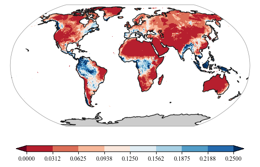
file_name='data/train/prcp.tif'
ds=xr.open_dataset(file_name)
data = ds['band_data'][7]
fig = plt.figure()
proj = ccrs.Robinson() #ccrs.Robinson()ccrs.Mollweide()Mollweide()
ax = fig.add_subplot(111, projection=proj)
levels = np.linspace(0, 0.25, num=9)
plot.one_map_flat(data, ax, levels=levels, cmap="RdBu", mask_ocean=False, add_coastlines=True, add_land=True, colorbar=True, plotfunc="pcolormesh")<cartopy.mpl.geocollection.GeoQuadMesh at 0x1c9263ca490>
# 创建二维矩阵
import random
matrix = torch.mean(torch.stack([torch.mean(precipitation_re, 1)], 1), 1).flatten()
# 将矩阵中值为NaN的元素置为0
matrix[torch.isnan(matrix)] = 0

# 获取所有不为NaN的元素的索引
non_negative_indices = torch.nonzero(matrix)
precipitation_re = precipitation_re[non_negative_indices.flatten(), :]
class Config(object):
t0 = 155 #155
t1 = 12
t = t0 + t1
train_num = 8000 #8
validation_num = 1000 #1
test_num = 1000 #1
in_channels = 1
batch_size = 500 #500 NSE 0.75
lr = .0005 # learning rate
epochs = 100import torch
import matplotlib.pyplot as plt
import numpy as np
from torch.utils.data import Dataset
class time_series_decoder_paper(Dataset):
"""synthetic time series dataset from section 5.1"""
def __init__(self,t0=120,N=4500,dx=None,dy=None,transform=None):
"""
Args:
t0: previous t0 data points to predict from
N: number of data points
transform: any transformations to be applied to time series
"""
self.t0 = t0
self.N = N
self.dx = dx
self.dy = dy
self.transform = None
# time points
#self.x = torch.cat(N*[torch.arange(0,t0+24).type(torch.float).unsqueeze(0)])
self.x = dx
self.fx = dy
# self.fx = torch.cat([A1.unsqueeze(1)*torch.sin(np.pi*self.x[0,0:12]/6)+72 ,
# A2.unsqueeze(1)*torch.sin(np.pi*self.x[0,12:24]/6)+72 ,
# A3.unsqueeze(1)*torch.sin(np.pi*self.x[0,24:t0]/6)+72,
# A4.unsqueeze(1)*torch.sin(np.pi*self.x[0,t0:t0+24]/12)+72],1)
# add noise
# self.fx = self.fx + torch.randn(self.fx.shape)
self.masks = self._generate_square_subsequent_mask(t0)
# print out shapes to confirm desired output
print("x: ",self.x.shape,
"fx: ",self.fx.shape)
def __len__(self):
return len(self.fx)
def __getitem__(self,idx):
if torch.is_tensor(idx):
idx = idx.tolist()
sample = (self.x[idx,:,:], #self.x[idx,:]
self.fx[idx,:],
self.masks)
if self.transform:
sample=self.transform(sample)
return sample
def _generate_square_subsequent_mask(self,t0):
mask = torch.zeros(Config.t,Config.t)
for i in range(0,Config.t0):
mask[i,Config.t0:] = 1
for i in range(Config.t0,Config.t):
mask[i,i+1:] = 1
mask = mask.float().masked_fill(mask == 1, float('-inf'))#.masked_fill(mask == 1, float(0.0))
return maskclass TransformerTimeSeries(torch.nn.Module):
"""
Time Series application of transformers based on paper
causal_convolution_layer parameters:
in_channels: the number of features per time point
out_channels: the number of features outputted per time point
kernel_size: k is the width of the 1-D sliding kernel
nn.Transformer parameters:
d_model: the size of the embedding vector (input)
PositionalEncoding parameters:
d_model: the size of the embedding vector (positional vector)
dropout: the dropout to be used on the sum of positional+embedding vector
"""
def __init__(self):
super(TransformerTimeSeries,self).__init__()
self.input_embedding = context_embedding(Config.in_channels+1,256,5)
self.positional_embedding = torch.nn.Embedding(512,256)
self.decode_layer = torch.nn.TransformerEncoderLayer(d_model=256,nhead=8)
self.transformer_decoder = torch.nn.TransformerEncoder(self.decode_layer, num_layers=3)
self.fc1 = torch.nn.Linear(256,1)
def forward(self,x,y,attention_masks):
# concatenate observed points and time covariate
# (B*feature_size*n_time_points)
#re z = torch.cat((y.unsqueeze(1),x.unsqueeze(1)),1)
z = torch.cat((y,x),1)
# input_embedding returns shape (Batch size,embedding size,sequence len) -> need (sequence len,Batch size,embedding_size)
#re z_embedding = self.input_embedding(z).permute(2,0,1)
z_embedding = self.input_embedding(z).unsqueeze(1).permute(3, 1, 0, 2)
# get my positional embeddings (Batch size, sequence_len, embedding_size) -> need (sequence len,Batch size,embedding_size)
x1 = x.type(torch.long)
x1[x1 < 0] = 0
positional_embeddings = self.positional_embedding(x1).permute(2, 1, 0, 3)
#re #positional_embeddings = self.positional_embedding(x.type(torch.long)).permute(1,0,2)
input_embedding = z_embedding+positional_embeddings
input_embedding1 = torch.mean(input_embedding, 1)
transformer_embedding = self.transformer_decoder(input_embedding1,attention_masks)
output = self.fc1(transformer_embedding.permute(1,0,2))
return output
import torch
import numpy as np
import matplotlib.pyplot as plt
import torch.nn.functional as F
class CausalConv1d(torch.nn.Conv1d):
def __init__(self,
in_channels,
out_channels,
kernel_size,
stride=1,
dilation=1,
groups=1,
bias=True):
super(CausalConv1d, self).__init__(
in_channels,
out_channels,
kernel_size=kernel_size,
stride=stride,
padding=0,
dilation=dilation,
groups=groups,
bias=bias)
self.__padding = (kernel_size - 1) * dilation
def forward(self, input):
return super(CausalConv1d, self).forward(F.pad(input, (self.__padding, 0)))
class context_embedding(torch.nn.Module):
def __init__(self,in_channels=Config.in_channels,embedding_size=256,k=5):
super(context_embedding,self).__init__()
self.causal_convolution = CausalConv1d(in_channels,embedding_size,kernel_size=k)
def forward(self,x):
x = self.causal_convolution(x)
return torch.tanh(x)class LSTM_Time_Series(torch.nn.Module):
def __init__(self,input_size=2,embedding_size=256,kernel_width=9,hidden_size=512):
super(LSTM_Time_Series,self).__init__()
self.input_embedding = context_embedding(input_size,embedding_size,kernel_width)
self.lstm = torch.nn.LSTM(embedding_size,hidden_size,batch_first=True)
self.fc1 = torch.nn.Linear(hidden_size,1)
def forward(self,x,y):
"""
x: the time covariate
y: the observed target
"""
# concatenate observed points and time covariate
# (B,input size + covariate size,sequence length)
# z = torch.cat((y.unsqueeze(1),x.unsqueeze(1)),1)
z_obs = torch.cat((y.unsqueeze(1),x.unsqueeze(1)),1)
if isLSTM:
z_obs = torch.cat((y, x),1)
# input_embedding returns shape (B,embedding size,sequence length)
z_obs_embedding = self.input_embedding(z_obs)
# permute axes (B,sequence length, embedding size)
z_obs_embedding = self.input_embedding(z_obs).permute(0,2,1)
# all hidden states from lstm
# (B,sequence length,num_directions * hidden size)
lstm_out,_ = self.lstm(z_obs_embedding)
# input to nn.Linear: (N,*,Hin)
# output (N,*,Hout)
return self.fc1(lstm_out)from torch.utils.data import DataLoader
import random
random.seed(0)
random_indices = random.sample(range(non_negative_indices.shape[0]), Config.train_num)
random_indices1 = random.sample(range(non_negative_indices.shape[0]), Config.validation_num)
random_indices2 = random.sample(range(non_negative_indices.shape[0]), Config.test_num)
dx = torch.stack([torch.cat(Config.train_num*[torch.arange(0,Config.t).type(torch.float).unsqueeze(0)]).cuda()], 1)
dx1 = torch.stack([torch.cat(Config.validation_num*[torch.arange(0,Config.t).type(torch.float).unsqueeze(0)]).cuda()], 1)
dx2 = torch.stack([torch.cat(Config.test_num*[torch.arange(0,Config.t).type(torch.float).unsqueeze(0)]).cuda()], 1)
train_dataset = time_series_decoder_paper(t0=Config.t0,N=Config.train_num,dx=dx ,dy=precipitation_re[np.array([random_indices]).flatten(),0:Config.t].unsqueeze(1))
validation_dataset = time_series_decoder_paper(t0=Config.t0,N=Config.validation_num,dx=dx1,dy=precipitation_re[np.array([random_indices1]).flatten(),0:Config.t].unsqueeze(1))
test_dataset = time_series_decoder_paper(t0=Config.t0,N=Config.test_num,dx=dx2,dy=precipitation_re[np.array([random_indices2]).flatten(),0:Config.t].unsqueeze(1))x: torch.Size([8000, 1, 167]) fx: torch.Size([8000, 1, 167])
x: torch.Size([1000, 1, 167]) fx: torch.Size([1000, 1, 167])
x: torch.Size([1000, 1, 167]) fx: torch.Size([1000, 1, 167])
criterion = torch.nn.MSELoss()
train_dl = DataLoader(train_dataset,batch_size=Config.batch_size,shuffle=True, generator=torch.Generator(device='cpu'))
validation_dl = DataLoader(validation_dataset,batch_size=Config.batch_size, generator=torch.Generator(device='cpu'))
test_dl = DataLoader(test_dataset,batch_size=Config.batch_size, generator=torch.Generator(device='cpu'))
criterion_LSTM = torch.nn.MSELoss()LSTM = LSTM_Time_Series().cuda()def Dp(y_pred,y_true,q):
return max([q*(y_pred-y_true),(q-1)*(y_pred-y_true)])
def Rp_num_den(y_preds,y_trues,q):
numerator = np.sum([Dp(y_pred,y_true,q) for y_pred,y_true in zip(y_preds,y_trues)])
denominator = np.sum([np.abs(y_true) for y_true in y_trues])
return numerator,denominator
def train_epoch(LSTM,train_dl,t0=Config.t0):
LSTM.train()
train_loss = 0
n = 0
for step,(x,y,_) in enumerate(train_dl):
x = x.cuda()
y = y.cuda()
optimizer.zero_grad()
output = LSTM(x,y)
loss = criterion(output.squeeze()[:,(Config.t0-1):(Config.t0+Config.t1-1)],y.cuda()[:,0,Config.t0:])
loss.backward()
optimizer.step()
train_loss += (loss.detach().cpu().item() * x.shape[0])
n += x.shape[0]
return train_loss/n
def eval_epoch(LSTM,validation_dl,t0=Config.t0):
LSTM.eval()
eval_loss = 0
n = 0
with torch.no_grad():
for step,(x,y,_) in enumerate(train_dl):
x = x.cuda()
y = y.cuda()
output = LSTM(x,y)
loss = criterion(output.squeeze()[:,(Config.t0-1):(Config.t0+Config.t1-1)],y.cuda()[:,0,Config.t0:])
eval_loss += (loss.detach().cpu().item() * x.shape[0])
n += x.shape[0]
return eval_loss/n
def test_epoch(LSTM,test_dl,t0=Config.t0):
with torch.no_grad():
predictions = []
observations = []
LSTM.eval()
for step,(x,y,_) in enumerate(train_dl):
x = x.cuda()
y = y.cuda()
output = LSTM(x,y)
for p,o in zip(output.squeeze()[:,(Config.t0-1):(Config.t0+Config.t1-1)].cpu().numpy().tolist(),y.cuda()[:,0,Config.t0:].cpu().numpy().tolist()):
predictions.append(p)
observations.append(o)
num = 0
den = 0
for y_preds,y_trues in zip(predictions,observations):
num_i,den_i = Rp_num_den(y_preds,y_trues,.5)
num+=num_i
den+=den_i
Rp = (2*num)/den
return Rptrain_epoch_loss = []
eval_epoch_loss = []
Rp_best = 30
isLSTM = True
optimizer = torch.optim.Adam(LSTM.parameters(), lr=Config.lr)
for e,epoch in enumerate(range(Config.epochs)):
train_loss = []
eval_loss = []
l_train = train_epoch(LSTM,train_dl)
train_loss.append(l_train)
l_eval = eval_epoch(LSTM,validation_dl)
eval_loss.append(l_eval)
Rp = test_epoch(LSTM,test_dl)
if Rp_best > Rp:
Rp_best = Rp
with torch.no_grad():
print("Epoch {}: Train loss={} \t Eval loss = {} \t Rp={}".format(e,np.mean(train_loss),np.mean(eval_loss),Rp))
train_epoch_loss.append(np.mean(train_loss))
eval_epoch_loss.append(np.mean(eval_loss))Epoch 0: Train loss=1.169178232550621 Eval loss = 1.0225972533226013 Rp=0.9754564549482763
Epoch 1: Train loss=1.0208212696015835 Eval loss = 1.0133976340293884 Rp=0.992397172460293
Epoch 2: Train loss=1.0135348699986935 Eval loss = 1.0102826319634914 Rp=1.0010193148701694
Epoch 3: Train loss=1.0075771994888783 Eval loss = 1.003737311810255 Rp=0.9874602462009079
Epoch 4: Train loss=0.9986509047448635 Eval loss = 0.991193663328886 Rp=0.9851476850727866
Epoch 5: Train loss=0.9815127141773701 Eval loss = 0.9676672779023647 Rp=0.9776791701859356
Epoch 6: Train loss=0.9377330988645554 Eval loss = 0.8851083293557167 Rp=0.9021427715861259
Epoch 7: Train loss=0.8124373629689217 Eval loss = 0.776776347309351 Rp=0.8164312307396333
Epoch 8: Train loss=0.7808051072061062 Eval loss = 0.7724409475922585 Rp=0.8044285279275872
Epoch 9: Train loss=0.7723440378904343 Eval loss = 0.7691570967435837 Rp=0.8276665115435272
Epoch 10: Train loss=0.7680666074156761 Eval loss = 0.7604397684335709 Rp=0.8172812960763582
Epoch 11: Train loss=0.7637499608099461 Eval loss = 0.7642757333815098 Rp=0.7958800149846623
Epoch 12: Train loss=0.7604391016066074 Eval loss = 0.7545832060277462 Rp=0.7959258052455023
Epoch 13: Train loss=0.7542793937027454 Eval loss = 0.758263424038887 Rp=0.8029712542553213
Epoch 14: Train loss=0.7513296827673912 Eval loss = 0.74464987590909 Rp=0.7928307957450957
Epoch 15: Train loss=0.7609197050333023 Eval loss = 0.7561161443591118 Rp=0.7961394733618599
Epoch 16: Train loss=0.7611901015043259 Eval loss = 0.754481915384531 Rp=0.8042048513261087
Epoch 17: Train loss=0.7494660168886185 Eval loss = 0.7436127960681915 Rp=0.808727372545216
Epoch 18: Train loss=0.7624928876757622 Eval loss = 0.7601931132376194 Rp=0.8278642644450237
Epoch 19: Train loss=0.7445684559643269 Eval loss = 0.7404011972248554 Rp=0.7988691222148593
Epoch 20: Train loss=0.7364756055176258 Eval loss = 0.7331099547445774 Rp=0.7900263164250347
Epoch 21: Train loss=0.7366516776382923 Eval loss = 0.7335694879293442 Rp=0.7858690993104261
Epoch 22: Train loss=0.7310461960732937 Eval loss = 0.7295852825045586 Rp=0.7947732982354974
Epoch 23: Train loss=0.7325067669153214 Eval loss = 0.7321035303175449 Rp=0.7994415259947144
Epoch 24: Train loss=0.7324810847640038 Eval loss = 0.7215580977499485 Rp=0.7793204264401973
Epoch 25: Train loss=0.7343184538185596 Eval loss = 0.7716133445501328 Rp=0.8319286623223218
Epoch 26: Train loss=0.7366975098848343 Eval loss = 0.7249130606651306 Rp=0.77453832290699
Epoch 27: Train loss=0.7278863601386547 Eval loss = 0.720306035131216 Rp=0.7780187017935781
Epoch 28: Train loss=0.7243384085595608 Eval loss = 0.715414222329855 Rp=0.7660441378673354
Epoch 29: Train loss=0.7391963303089142 Eval loss = 0.8104664944112301 Rp=0.848384596737658
Epoch 30: Train loss=0.7501446716487408 Eval loss = 0.7330859526991844 Rp=0.7958694240958736
Epoch 31: Train loss=0.7319861426949501 Eval loss = 0.7288344763219357 Rp=0.7764215311271584
Epoch 32: Train loss=0.7289896085858345 Eval loss = 0.7186561860144138 Rp=0.7719541082002876
Epoch 33: Train loss=0.7208635434508324 Eval loss = 0.7130853533744812 Rp=0.7693201078171342
Epoch 34: Train loss=0.7188350297510624 Eval loss = 0.7184220626950264 Rp=0.7790605390063141
Epoch 35: Train loss=0.7278616651892662 Eval loss = 0.7226458676159382 Rp=0.7934061207417414
Epoch 36: Train loss=0.7257222011685371 Eval loss = 0.7461872175335884 Rp=0.8043810986938649
Epoch 37: Train loss=0.722360011190176 Eval loss = 0.7184372805058956 Rp=0.7733680838057659
Epoch 38: Train loss=0.7406770437955856 Eval loss = 0.7328226044774055 Rp=0.7792520400962948
Epoch 39: Train loss=0.7231648564338684 Eval loss = 0.7170744873583317 Rp=0.7745043319879358
Epoch 40: Train loss=0.7179877758026123 Eval loss = 0.7121099643409252 Rp=0.7665604319856079
Epoch 41: Train loss=0.7204379811882973 Eval loss = 0.7137661874294281 Rp=0.7697876723151911
Epoch 42: Train loss=0.7189657613635063 Eval loss = 0.7145831622183323 Rp=0.7683013184528533
Epoch 43: Train loss=0.7236194014549255 Eval loss = 0.7213072367012501 Rp=0.7794286898969346
Epoch 44: Train loss=0.7113666497170925 Eval loss = 0.7064446061849594 Rp=0.7730508504910318
Epoch 45: Train loss=0.7169638313353062 Eval loss = 0.7072659730911255 Rp=0.7818726340368028
Epoch 46: Train loss=0.7137239314615726 Eval loss = 0.7547547481954098 Rp=0.8419246011202801
Epoch 47: Train loss=0.7260657027363777 Eval loss = 0.7107443884015083 Rp=0.7655332919045247
Epoch 48: Train loss=0.7079816907644272 Eval loss = 0.7071417346596718 Rp=0.773454930517809
Epoch 49: Train loss=0.7094167955219746 Eval loss = 0.7058326154947281 Rp=0.7727462602735332
Epoch 50: Train loss=0.7380903214216232 Eval loss = 0.7227592132985592 Rp=0.769177665270142
Epoch 51: Train loss=0.7130068391561508 Eval loss = 0.7105456776916981 Rp=0.7592860561025371
Epoch 52: Train loss=0.7084374688565731 Eval loss = 0.7031594552099705 Rp=0.7660899650703171
Epoch 53: Train loss=0.7042888924479485 Eval loss = 0.7040572166442871 Rp=0.7721988413128251
Epoch 54: Train loss=0.7063969075679779 Eval loss = 0.6986251175403595 Rp=0.7695131487850577
Epoch 55: Train loss=0.7053375691175461 Eval loss = 0.7212032824754715 Rp=0.7735872477697779
Epoch 56: Train loss=0.7035926096141338 Eval loss = 0.7097134478390217 Rp=0.784710594937848
Epoch 57: Train loss=0.735156461596489 Eval loss = 0.8654714487493038 Rp=0.911015246823642
Epoch 58: Train loss=0.8107807412743568 Eval loss = 0.7581384815275669 Rp=0.8157151369086734
Epoch 59: Train loss=0.7544550113379955 Eval loss = 0.7499602921307087 Rp=0.7949385155087615
Epoch 60: Train loss=0.746234655380249 Eval loss = 0.7389007620513439 Rp=0.7862202786182774
Epoch 61: Train loss=0.7351461201906204 Eval loss = 0.7316578552126884 Rp=0.7699839364702437
Epoch 62: Train loss=0.7276912368834019 Eval loss = 0.7233806289732456 Rp=0.7752237105789992
Epoch 63: Train loss=0.7192910276353359 Eval loss = 0.7333457358181477 Rp=0.7724518923905164
Epoch 64: Train loss=0.7260234951972961 Eval loss = 0.7129928097128868 Rp=0.7660325583116143
Epoch 65: Train loss=0.7277122773230076 Eval loss = 0.7464463748037815 Rp=0.7795688062338593
Epoch 66: Train loss=0.7259447425603867 Eval loss = 0.7074765078723431 Rp=0.7646423879285662
Epoch 67: Train loss=0.7121074683964252 Eval loss = 0.7206148467957973 Rp=0.7670712925578708
Epoch 68: Train loss=0.7051395028829575 Eval loss = 0.7368365041911602 Rp=0.8174581520496608
Epoch 69: Train loss=0.7655579410493374 Eval loss = 0.7538384310901165 Rp=0.7762011659936345
Epoch 70: Train loss=0.7304071560502052 Eval loss = 0.7248818911612034 Rp=0.791938228314532
Epoch 71: Train loss=0.7145950980484486 Eval loss = 0.7085471898317337 Rp=0.771219627305778
Epoch 72: Train loss=0.705636128783226 Eval loss = 0.7026742734014988 Rp=0.7582436097165333
Epoch 73: Train loss=0.7039311081171036 Eval loss = 0.701056282967329 Rp=0.7621456124101622
Epoch 74: Train loss=0.7022229805588722 Eval loss = 0.7022544406354427 Rp=0.7572908772835294
Epoch 75: Train loss=0.7077537477016449 Eval loss = 0.7068974897265434 Rp=0.7689672806983037
Epoch 76: Train loss=0.70463952049613 Eval loss = 0.7016653120517731 Rp=0.7620379826248179
Epoch 77: Train loss=0.6936824433505535 Eval loss = 0.6882451064884663 Rp=0.7536649577052977
Epoch 78: Train loss=0.7085927426815033 Eval loss = 0.7006802186369896 Rp=0.7573836578425687
Epoch 79: Train loss=0.6964434124529362 Eval loss = 0.6970510184764862 Rp=0.7566034081453576
Epoch 80: Train loss=0.7041287049651146 Eval loss = 0.7041221261024475 Rp=0.7517282641309433
Epoch 81: Train loss=0.7040938474237919 Eval loss = 0.694716889411211 Rp=0.7518976134462692
Epoch 82: Train loss=0.6934744939208031 Eval loss = 0.6876317113637924 Rp=0.7490530317847554
Epoch 83: Train loss=0.6924876533448696 Eval loss = 0.7114526480436325 Rp=0.7712103875056127
Epoch 84: Train loss=0.70367331802845 Eval loss = 0.6974217854440212 Rp=0.7550885913055979
Epoch 85: Train loss=0.7047922983765602 Eval loss = 0.6882399097084999 Rp=0.7489761214479039
Epoch 86: Train loss=0.6913500241935253 Eval loss = 0.6827207766473293 Rp=0.744314955284494
Epoch 87: Train loss=0.6916158571839333 Eval loss = 0.6919064372777939 Rp=0.7509365031084853
Epoch 88: Train loss=0.6971654705703259 Eval loss = 0.6914562620222569 Rp=0.7441346646542655
Epoch 89: Train loss=0.6963543370366096 Eval loss = 0.691758755594492 Rp=0.7572971481054963
Epoch 90: Train loss=0.6917684748768806 Eval loss = 0.6856491975486279 Rp=0.7448740185296933
Epoch 91: Train loss=0.6941814571619034 Eval loss = 0.6949076354503632 Rp=0.7525349231139533
Epoch 92: Train loss=0.69602020829916 Eval loss = 0.7147903628647327 Rp=0.7746622771469637
Epoch 93: Train loss=0.6934036538004875 Eval loss = 0.689013235270977 Rp=0.7674142639047323
Epoch 94: Train loss=0.6828178651630878 Eval loss = 0.6839329451322556 Rp=0.749017388184114
Epoch 95: Train loss=0.6820085123181343 Eval loss = 0.679760005325079 Rp=0.7496224481291669
Epoch 96: Train loss=0.6940162815153599 Eval loss = 0.6897397376596928 Rp=0.7505375270808133
Epoch 97: Train loss=0.6879976131021976 Eval loss = 0.7038531377911568 Rp=0.7740689357717414
Epoch 98: Train loss=0.6902556456625462 Eval loss = 0.6736902967095375 Rp=0.7441236415340688
Epoch 99: Train loss=0.6990400142967701 Eval loss = 0.7069363221526146 Rp=0.7699857686313047
import os
os.environ["KMP_DUPLICATE_LIB_OK"]="TRUE"
n_plots = 5

t0=120
with torch.no_grad():
    LSTM.eval()
    for step,(x,y,_) in enumerate(test_dl):
        x = x.cuda()
        y = y.cuda()

        output = LSTM(x,y)


        if step > n_plots:
            break

        with torch.no_grad():
            plt.figure(figsize=(10,10))
            plt.plot(x[1, 0].cpu().detach().squeeze().numpy(),y[1].cpu().detach().squeeze().numpy(),'g--',linewidth=3)
            plt.plot(x[1, 0, Config.t0:].cpu().detach().squeeze().numpy(),output[1,(Config.t0-1):(Config.t0+Config.t1-1),0].cpu().detach().squeeze().numpy(),'b--',linewidth=3)

            plt.xlabel("x",fontsize=20)
            plt.legend(["$[0,t_0+24)_{obs}$","$[t_0,t_0+24)_{predicted}$"])
            plt.show()


matrix = torch.empty(0).cuda()
obsmat = torch.empty(0).cuda()

with torch.no_grad():
    LSTM.eval()
    predictions = []
    observations = []
    for step,(x,y,attention_masks) in enumerate(test_dl):
        # if step == 8:
        #     break
        output = LSTM(x.cuda(),y.cuda())
        matrix = torch.cat((matrix, output.cuda()))
        obsmat = torch.cat((obsmat, y.cuda()))

pre = matrix.cpu().detach().numpy()
obs = obsmat.cpu().detach().numpy()
# libraries
import matplotlib.pyplot as plt
import numpy as np
import pandas as pd

# data
df = pd.DataFrame({
  'obs': obs[:, 0, Config.t0:Config.t].flatten(),
  'pre': pre[:, Config.t0:Config.t, 0].flatten()
})
df
<style scoped>
.dataframe tbody tr th:only-of-type {
vertical-align: middle;
}
</style>
.dataframe tbody tr th {
    vertical-align: top;
}

.dataframe thead th {
    text-align: right;
}
| obs | pre | |
|---|---|---|
| 0 | 1.195594 | 1.645856 |
| 1 | 1.649769 | 0.247605 |
| 2 | -0.608017 | -0.466307 |
| 3 | -0.471923 | -0.499275 |
| 4 | -1.097827 | -0.693097 |
| ... | ... | ... |
| 11995 | 3.649456 | 0.124768 |
| 11996 | -0.162433 | -0.615067 |
| 11997 | -0.589042 | -0.838524 |
| 11998 | -0.578971 | -0.815273 |
| 11999 | -0.744391 | -0.398436 |
12000 rows × 2 columns
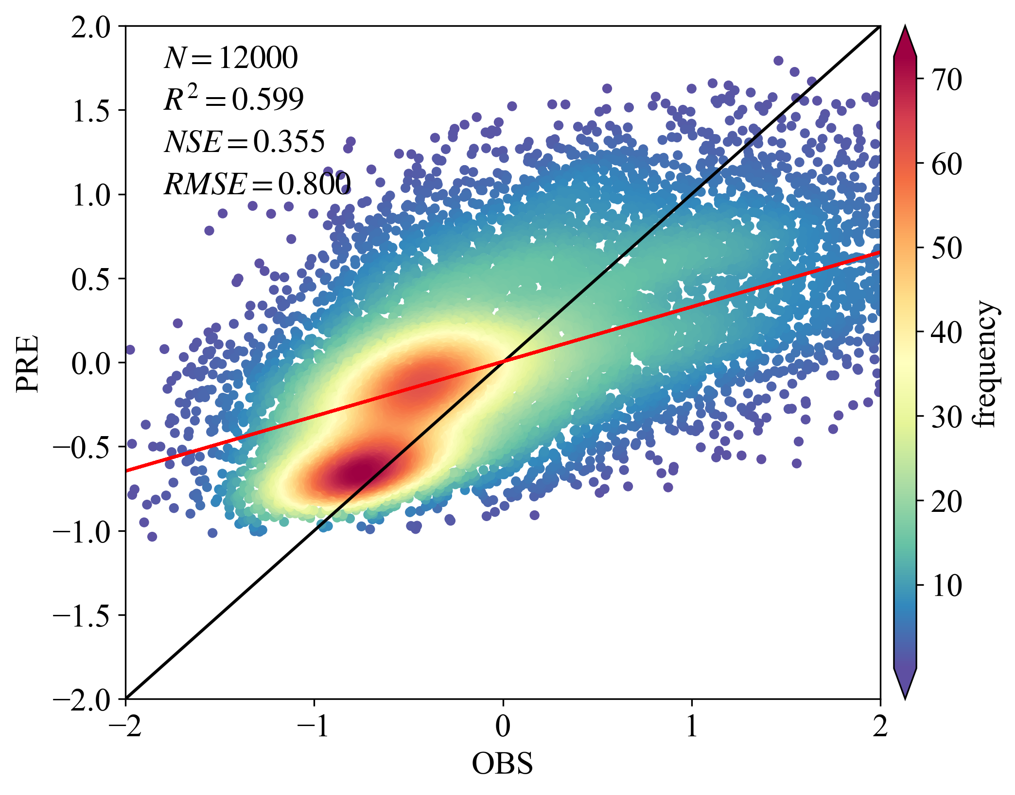
import numpy as np
import pandas as pd
import matplotlib.pyplot as plt
from scipy import stats
from matplotlib import rcParams
from statistics import mean
from sklearn.metrics import explained_variance_score,r2_score,median_absolute_error,mean_squared_error,mean_absolute_error
from scipy.stats import pearsonr
# 加载数据(PS:原始数据太多,采样10000)
# 默认是读取csv/xlsx的列成DataFrame


config = {"font.family":'Times New Roman',"font.size": 16,"mathtext.fontset":'stix'}
#df = df.sample(5000)
# 用于计算指标
x = df['obs']; y = df['pre']
rcParams.update(config)
BIAS = mean(x - y)
MSE = mean_squared_error(x, y)
RMSE = np.power(MSE, 0.5)
R2 = pearsonr(x, y).statistic
adjR2 = 1-((1-r2_score(x,y))*(len(x)-1))/(len(x)-Config.in_channels-1)
MAE = mean_absolute_error(x, y)
EV = explained_variance_score(x, y)
NSE = 1 - (RMSE ** 2 / np.var(x))
# 计算散点密度
xy = np.vstack([x, y])
z = stats.gaussian_kde(xy)(xy)
idx = z.argsort()
x, y, z = x.iloc[idx], y.iloc[idx], z[idx]

# 拟合(若换MK,自行操作)最小二乘
def slope(xs, ys):
    m = (((mean(xs) * mean(ys)) - mean(xs * ys)) / ((mean(xs) * mean(xs)) - mean(xs * xs)))
    b = mean(ys) - m * mean(xs)
    return m, b
k, b = slope(x, y)
regression_line = []
for a in x:
    regression_line.append((k * a) + b)

# 绘图,可自行调整颜色等等
import os
os.environ["KMP_DUPLICATE_LIB_OK"]="TRUE"

fig,ax=plt.subplots(figsize=(8,6),dpi=300)
scatter=ax.scatter(x, y, marker='o', c=z*100, edgecolors=None ,s=15, label='LST',cmap='Spectral_r')
cbar=plt.colorbar(scatter,shrink=1,orientation='vertical',extend='both',pad=0.015,aspect=30,label='frequency')
plt.plot([-30,30],[-30,30],'black',lw=1.5)  # 画的1:1线,线的颜色为black,线宽为0.8
plt.plot(x,regression_line,'red',lw=1.5)      # 预测与实测数据之间的回归线
plt.axis([-30,30,-30,30])  # 设置线的范围
plt.xlabel('OBS',family = 'Times New Roman')
plt.ylabel('PRE',family = 'Times New Roman')
plt.xticks(fontproperties='Times New Roman')
plt.yticks(fontproperties='Times New Roman')
plt.text(-1.8,1.75, '$N=%.f$' % len(y), family = 'Times New Roman') # text的位置需要根据x,y的大小范围进行调整。
plt.text(-1.8,1.50, '$R^2=%.3f$' % R2, family = 'Times New Roman')
plt.text(-1.8,1.25, '$NSE=%.3f$' % NSE, family = 'Times New Roman')

plt.text(-1.8,1, '$RMSE=%.3f$' % RMSE, family = 'Times New Roman')
plt.xlim(-2,2)                                  # 设置x坐标轴的显示范围
plt.ylim(-2,2)                                  # 设置y坐标轴的显示范围
plt.show()