This package offers an implementation of Gaussian dynamic Bayesian networks (GDBN) structure learning and inference based partially on Marco Scutari’s package bnlearn (https://www.bnlearn.com/). It also allows the construction of higher-order DBNs. Three structure learning algorithms are implemented:
- A variation on Ghada Trabelsi’s dynamic max-min hill climbing (https://theses.hal.science/tel-00996061/document).
- A particle swarm optimization algorithm for higher-order DBNs (https://doi.org/10.1109/BRC.2014.6880957)
- A scalable, order invariant particle swarm optimization algorithm for higher-order DBNs (https://link.springer.com/chapter/10.1007/978-3-030-86271-8_14)
Inference is performed either via the particle filtering offered by bnlearn or by doing exact inference over the multivariate Gaussian equivalent of a network implemented in this package. A visualization tool is also implemented for GDBNs and bnlearn’s BNs via the visNetwork package (https://github.com/datastorm-open/visNetwork).
The main functionality of the package is running and working. In order of importance, the next objectives are:
- To refractor the DMMHC algorithm into R6 for consistency with the PSOHO algorithm and with any new structure learning algorithms.
- To add an automatically generated shiny interface of the net. This makes interacting with the network easier and allows for simulation prototypes.
For now, the dbn.fit object as an extension of bnlearn’s bn.fit object will stay the same except for the “mu” and “sigma” attributes added to it. This way, it remains easy to call bnlearn’s methods on the dbn.fit object and I can store the MVN transformation inside the same object. Not an elegant solution, but its simplicity is enough. What should be addressed is having to perform the folding of a dataset outside the predict function.
This package requires R ≥ 3.6.1 to work properly. It also works for R ≥ 3.5.0, the only difference is the color palette of the DBN visualization tool.
The bnlearn and data.table packages, among others, are required for this package to work. They will be installed automatically when installing this package. They can also be installed manually via CRAN with the command
install.packages(c("bnlearn", "data.table"))The packages visNetwork, magrittr and grDevices are optional for the visualization tool. They will only be required if you want to use it.
As of today, the easiest way of installing dbnR is via CRAN. To install it, simply run
install.packages('dbnR')You can also install the latest version in GitHub with the install_github function in the devtools package. The commands you need to run are
library(devtools)
devtools::install_github("dkesada/dbnR")
This will install the required dependencies if they are not available. After this, you will be ready to use the package.
To get the structure of a GDBN from a dataset, you need to use the function learn_dbn_struc
library(dbnR)
#> Cargando paquete requerido: bnlearn
#>
#> Adjuntando el paquete: 'dbnR'
#> The following objects are masked from 'package:bnlearn':
#>
#> degree, nodes, nodes<-, scoredata(motor)
size <- 3
dt_train <- motor[200:2500]
dt_val <- motor[2501:3000]
net <- learn_dbn_struc(dt_train, size)The dt argument has to be either a data.frame or a data.table of numeric columns, in the example we use the sample dataset included in the package. The size argument determines the number of time slices that your net is going to have, that is, the Markovian order of the net. A Markovian order of 1 means that your data in the present is independent of the past given the previous time slice. If your case doesn’t meet this criteria, the size of the net can be increased, to take into account more past time slices in the inference. In our function, Markovian order = size - 1. The function returns a ‘dbn’ object that inherits from the ‘bn’ class in bnlearn, so that its auxiliary functions like ‘arcs’ and such also work on DBN structures.
Once the structure is learnt, it can be plotted and used to learn the parameters
plot_dynamic_network(net)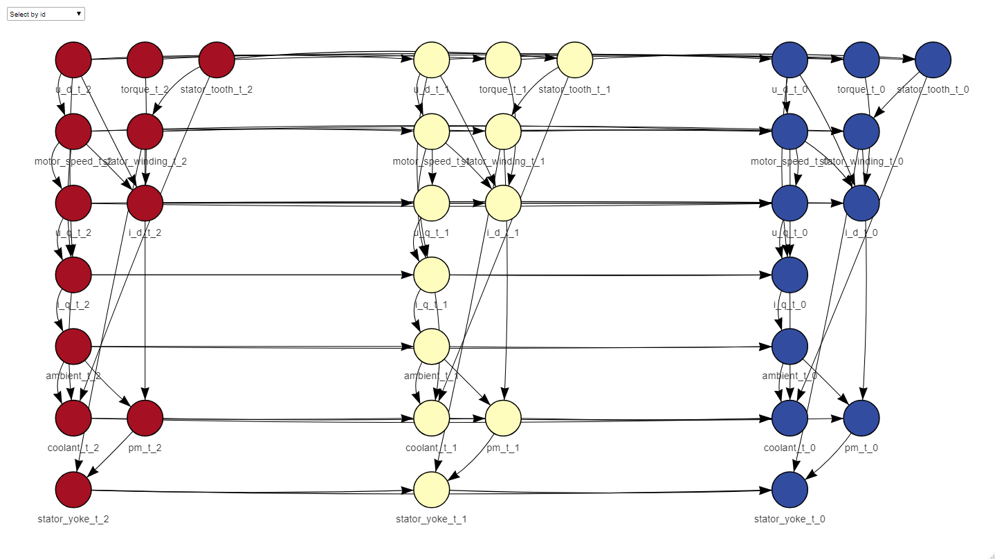
f_dt_train <- fold_dt(dt_train, size)
fit <- fit_dbn_params(net, f_dt_train, method = "mle-g")
After learning the net, two different types of inference can be performed: point-wise inference over a dataset and forecasting to some horizon. Point-wise inference uses the folded dt to try and predict the objective variables in each row. Forecasting to some horizon, on the other hand, tries to predict the behaviour in the future M instants given some initial evidence of the variables.
There is an extensive example of how to use the package in the markdowns folder, which covers more advanced concepts of structure learning and inference.
This project is licensed under the GPL-3 License, following on bnlearn’s GPL(≥ 2) license.
- The bnlearn package (https://www.bnlearn.com/).
- The visNetwork package (https://datastorm-open.github.io/visNetwork/)
- Kaggle’s dataset repository, where the sample dataset is from (https://kaggle.com/datasets/wkirgsn/electric-motor-temperature)
- Koller, D., & Friedman, N. (2009). Probabilistic graphical models: principles and techniques. MIT press.
- Murphy, K. P. (2012). Machine learning: a probabilistic perspective. MIT press.
-
Quesada, D., Valverde, G., Larrañaga, P., & Bielza, C. (2021). Long-term forecasting of multivariate time series in industrial furnaces with dynamic Gaussian Bayesian networks. Engineering Applications of Artificial Intelligence, 103, 104301.
-
Quesada, D., Bielza, C., & Larrañaga, P. (2021, September). Structure Learning of High-Order Dynamic Bayesian Networks via Particle Swarm Optimization with Order Invariant Encoding. In International Conference on Hybrid Artificial Intelligence Systems (pp. 158-171). Springer, Cham.
-
Quesada, D., Bielza, C., Fontán, P., & Larrañaga, P. (2022). Piecewise forecasting of nonlinear time series with model tree dynamic Bayesian networks. International Journal of Intelligent Systems, 37, 9108-9137.


