In Supervised Learning, the model is trained on labeled data, with clear input-output associations. This enables the algorithm to make predictions or take actions based on both labeled and future unlabeled data.

1. Labeled Data: Each training example includes input features and a corresponding output label. For instance, in a "Spam vs. Ham" email classifier, features could be email text and metadata, with labels marking emails as "spam" or "not spam" (ham).

2. Objective: The primary task is often predictive, such as identifying classes or values (Classification, Regression). The goal is to minimize the difference between predicted and actual labels.

3. Model Feedback: Through an evaluative process, the algorithm adjusts its parameters to improve accuracy. This mechanism is termed the "feedback loop."

4. Generalization: A key goal is for the algorithm to accurately predict labels on unseen data, not just on the training set.

5. Predictive Power: The model learns to make predictions or decisions based on input data, which is different from unsupervised learning where the focus is more on discovering hidden patterns or structures in the data.

6. Human Involvement: Supervised learning often requires humans to provide both input-output pairs for training and to assess model performance.

7. Training and Testing: The labeled data is typically divided into two sets—training and testing—to gauge model performance. More advanced techniques, like k-fold cross-validation, can also be employed for better accuracy assessment, especially in situations with limited data availability.

8. Direct Feedback: Often used to drive specific outcomes, supervised models result in direct and interpretable outputs (e.g., "The loan should be approved" or "The image is of a cat").

• Finance: Credit scoring, fraud detection, and stock price forecasting.
• Healthcare: Medical diagnostics, drug discovery, and personalized treatment plans.
• Marketing: Customer segmentation, recommendation engines, and churn prediction.
• Security: Biometric identification, threat detection, and object recognition in surveillance systems.
• Text and Voice Recognition: Sentiment analysis, speech-to-text, and chatbots.

• Interpretability: Supervised learning models are often easier to interpret due to the direct relationship between input and output.
• Customizability: The ability to label data according to specific business needs makes these models highly customizable.
• High Accuracy: With precisely labeled data for training, supervised models can reach high levels of accuracy.
• Informative Features: They can provide insights into which features are most influential in the prediction.

• Data and Labeling Requirements: The need for labeled data can be a significant challenge, especially with more specialized tasks.
• Potential Bias: Models can inherit biases from labeled data, leading to unfair or inaccurate predictions.
• Lack of Flexibility: If labeled data changes or new classes/outcomes appear, the algorithm needs to be retrained.

• Data Quality Matters Most: The level of success in supervised learning largely depends on the quality of labeled data.
• Understand Your Task: Choose the correct model based on the inherently known target variable or the task, whether classification or regression.
• Model Tuning: Mechanisms such as hyperparameter tuning can further enhance model performance.
• Avoid Overfitting: Strive for a model that can generalize well to unseen data.

Here is the Python code:

# Import necessary libraries
from sklearn.model_selection import train_test_split
from sklearn.feature_extraction.text import TfidfVectorizer
from sklearn.svm import SVC
from sklearn.metrics import accuracy_score, classification_report

# Assuming 'X' is a list of emails and 'y' contains corresponding labels
# Split the dataset into training and testing sets
X_train, X_test, y_train, y_test = train_test_split(X, y, test_size=0.3, random_state=42)

# Convert email text into numeric features using tf-idf
tfidf = TfidfVectorizer()
X_train_tfidf = tfidf.fit_transform(X_train)
X_test_tfidf = tfidf.transform(X_test)

# Instantiate and train a Support Vector Machine classifier
svm_classifier = SVC(kernel='linear')
svm_classifier.fit(X_train_tfidf, y_train)

# Make predictions on the test set and assess accuracy
y_pred = svm_classifier.predict(X_test_tfidf)
accuracy = accuracy_score(y_test, y_pred)
print(f"Test Set Accuracy: {accuracy:.2f}")

# Get a detailed performance report
print(classification_report(y_test, y_pred))

Supervised Learning and Unsupervised Learning are two primary paradigms in machine learning. They differ in data requirements, learning methods, and applications.

In Supervised Learning, the model is trained on labeled data, making it responsible for learning the mapping from input to output.

This discipline is characterized by:

• Training Dataset: A labeled dataset where both input and output are provided.
• Learning Objective: To minimize the discrepancy between predicted and actual outputs.
• Prediction Strategy: Based on previously seen examples.
• Applications: Vast, ranging from image recognition and text categorization to regression tasks.

• Classification: Utilized when the output is a category or a label, e.g., spam prediction.

  • Decision Trees, Random Forest, k-nearest neighbors (k-NN), Support Vector Machines (SVM)

• Regression: Ideal for predicting continuous-valued outputs, such as house prices.

  • Linear Regression, Polynomial Regression, Ridge Regression, Lasso Regression

• Sequence Generation: Used in sequential data tasks, providing future steps.

  • Recurrent Neural Networks (RNN), Long Short-Term Memory (LSTM)

• Time-Series Forecasting: Specialized in making predictions based on historical data.

  • Autoregressive Integrated Moving Average (ARIMA), Gradient Boosting Machines (GBM) including XGBoost and LightGBM

• Anomaly Detection: Identifies rare data points that can be indicative of errors.

  • One-Class SVM, Isolation Forest, Local Outlier Factor (LOF)

• Object Detection: Deals with locating and classifying objects within given images.

  • Faster R-CNN, You Only Look Once (YOLO)

Unsupervised Learning doesn't rely on labeled output data. Instead, it aims to extract meaningful patterns or structures from the input data alone.

This discipline is characterized by:

• Outcomes: Discovering hidden patterns, reducing dimensionality, and grouping data.
• Learning Paradigm: Self-organization based on data features.

• Clustering: Divides data into groups based on similarities.

  • k-Means, Hierarchical Clustering, DBSCAN

• Dimensionality Reduction: Focuses on compressing data into lower-dimensional spaces.

  • Principal Component Analysis (PCA), t-Distributed Stochastic Neighbor Embedding (t-SNE)

• Density Estimation: Determines the distribution of data within the feature space.

  • Gaussian Mixture Models (GMM), Kernel Density Estimation (KDE)

• Association Rule Learning: For discovering interesting relations between features in large datasets.

  • Apriori, Eclat

• Generative Adversarial Networks (GANs): A framework for generating data using two competing neural networks.

  • GANs, Variational Autoencoders (VAEs)

• Self-Organizing Maps (SOMs): Implementations of neural networks focused on clustering and visualization.

  • SOMs

• Expectation-Maximization (EM): A method used to estimate the parameters of statistical models even when there are unobserved data points.

  • Mixture models using EM for cluster estimation such as Gaussian Mixture Model (GMM)

While Hybrid Models integrate both supervised and unsupervised techniques, the learning is based on feedback from the environment or expertise from specialized domains.

This interaction often involves semi-structured datasets, where some data is labeled, and others are not. Techniques that blur the line between these two paradigms are known as semi-supervised.

• Semi-supervised Learning: Utilizes a combination of labeled and unlabeled data. Techniques focus on leveraging the collective information from both types.

  • Label Propagation, Co-Training

• Reinforcement Learning: The learning system, known as the agent, makes decisions within an environment, aiming to maximize some notion of cumulative reward.

  • Q-Learning, Deep Q-Networks (DQN)

Supervised Learning is used to tackle diverse problem types across domains like Healthcare, Finance, and Retail. Supervised learning tasks deal with labeled datasets where each data point comes with an associated target or outcome.

Let's explore the specific problem types and algorithms suited for them:

In classification, the goal is to categorize data points into distinct groups/classes. It's commonly utilized in email spam filters, image recognition, and medical diagnoses.

• Logistic Regression: Code example below.

from sklearn.linear_model import LogisticRegression

# Create an instance of the classifier
classifier = LogisticRegression()

# Train the model using the training data
classifier.fit(X_train, y_train)

# Predict the class labels for new data
y_pred = classifier.predict(X_test)

• K-Nearest Neighbors (KNN)
• Support Vector Machines (SVM)
• Decision Trees
• Random Forests
• Gradient Boosting

Regression focuses on predicting continuous values. It's used in scenarios such as real estate price prediction and demand forecasting.

• Linear Regression: Code example below.

from sklearn.linear_model import LinearRegression

# Create an instance of the regressor
regressor = LinearRegression()

# Fit the model to the training data
regressor.fit(X_train, y_train)

# Predict the target variable for new data
y_pred = regressor.predict(X_test)

• Support Vector Regression (SVR)
• Random Forest Regression
• Gradient Boosting

Here, the focus is on identifying rare events or observations that differ significantly from the norm. Anomaly detection is relevant in credit card fraud detection or identifying network intrusions.

• Isolation Forest
• k-means Clustering
• Autoencoders

Time series forecasting predicts future values of a variable based on historical data. It has applications in weather forecasting and stock market analysis.

• Autoregressive Integrated Moving Average (ARIMA)
• Long Short-Term Memory (LSTM)

Supervised learning is used in tasks like sentiment analysis, text classification, and named entity recognition.

• Support Vector Machines (SVM)
• Naive Bayes
• Recurrent Neural Networks (RNNs)

In these tasks, the goal is to identify and locate objects within an image. It's commonly found in self-driving cars and facial recognition systems.

• Convolutional Neural Networks (CNNs)
• Region-based Convolutional Neural Networks (R-CNNs)
• You Only Look Once (YOLO)

Recommender systems generate recommendations based on user behavior. They are commonly used by online retailers and streaming platforms.

• Collaborative Filtering
• Matrix Factorization

Generative models learn the underlying probability distribution of the data. They are commonly used in tasks such as image synthesis and natural language generation.

• Variational Autoencoders (VAEs)
• Generative Adversarial Networks (GANs)

In Supervised Learning, 'training datasets' are used to fit the model to the underlying data-generating processes. This enables the model to device generalized patterns that can be used to make predictions or decisions.

The 'testing datasets' are employed to assess the model's performance. The model makes predictions or classifications using unseen data points from the test set. This allows for an impartial evaluation of its capabilities.

The training dataset is the "teaching tool" for the model. It's composed of pairs of input data (features) and known corresponding output data (labels).

The objective during training is to reduce the generalization error, which is the expected error on new, unseen data. The training dataset is utilized in an iterative fashion to achieve this goal.

1. Fitting the Model: The model adjusts its parameters or structure to minimize the difference between its predictions and the true labels in the training dataset. This process is also known as optimization or learning.

2. Evaluating Performance: The model's current performance on the training data is assessed, typically using a predefined measure such as accuracy or mean squared error. This step helps determine how well the model is doing before making further adjustments.

3. Iterative Learning: Steps 1 and 2 are repeated multiple times, allowing the model to further refine its predictive ability.

Once the model "learns" from the training dataset, it is then validated or tested using the test dataset.

The testing dataset is the "examination paper" for the model. It is also divided into features and labels, much like the training dataset, but the labels are kept hidden from the model.

The primary function of the test dataset is to provide an unbiased evaluation of the model's predictive accuracy on new, unseen data. This helps avoid issues like overfitting.

1. Making Predictions: The model is used to make predictions or classifications for the test set's features.

2. Assessing Accuracy: The model's predictions are compared to the true labels of the test set. The agreement between the predictions and true labels provides a measure of model performance.

The metrics generated from the test set's performance, such as accuracy, precision, recall, or F1 score, give an indication of how well the model is expected to perform on new, unseen data. This allows for an assessment of its generalization ability.

In supervised learning, the role of a Loss Function is to quantify the disparity between predicted and actual outcomes, providing a measure of the algorithm's performance.

• Guidance: Directs algorithms towards more accurate predictions.
• Optimization: Forms the basis for methods such as Gradient Descent, helping refine model parameters.
• Evaluation: Measures a model's accuracy or error rate.

For classification tasks:

• Binary Classification: Employs functions like the Cross-Entropy Loss, adept at handling categorical outcomes.
• Multi-Class Classification: Loss functions like the Categorical Cross-Entropy can accommodate multiple outcome possibilities.

In regression tasks, the choice of loss function varies based on the type of prediction:

• Linear Regression: Mean Squared Error (MSE) is often the go-to choice, ensuring the predicted continuous value aligns with the actual one.

• Quantile Regression: It prioritizes specific quantiles of the data, making Median Absolute Error (MAE) the preferred loss function.

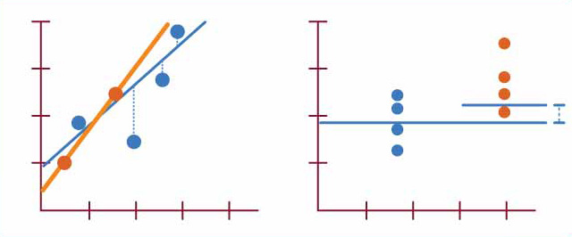
Overfitting and underfitting are two common pitfalls in machine learning models.

When a model overfits, it performs well on training data but poorly on unseen data. This is caused by the model being too complex for the given dataset. Such models tend to capture noise and outliers in the training data, leading to reduced generalization.

• High Model Complexity: Using models with many parameters, such as deep neural networks, can lead to overfitting.
• Insufficient Data: When the amount of available training data is limited, complex models are more prone to overfitting.

• The model has very high accuracy on the training set but much lower accuracy on the test set.
• Upon visualizing the model's performance, there might be a large divergence between training and test set accuracy or loss.

• Regularization: Techniques such as L1 or L2 regularization can discourage overfitting by penalizing large parameter values.
• Cross-Validation: Using techniques like k-fold cross-validation to estimate model performance more effectively.
• Feature Reduction: Reducing the number of input features can help simplify the model.

  from sklearn.linear_model import LogisticRegression
  model = LogisticRegression(penalty='l2', C=0.1)  # Example of L2 regularization

In underfitting, the model is too simplistic to capture the underlying patterns in the training data. This results in poor performance on both the training and test sets.

• Model Simplification: When using linear models to represent inherently non-linear relationships.
• Insufficient Training: When the training data is not representative of the true data distribution.

• The model has low accuracy on both the training and test sets.
• Visualizing the learning curves, one may observe that performance metrics have plateaued at a level well below the desired threshold.

• Model Complexity Increase: Employ more powerful models that can better capture complex patterns.
• Feature Engineering: Creating more informative features from the existing data.
• Extended Training: Giving the current model more training data can sometimes help.

  from sklearn.ensemble import RandomForestClassifier  # Example of a more complex model
  model = RandomForestClassifier()

Machine Learning is about striking a balance. The goal is to have a model that generalizes well to unseen data. This is achieved by:

1. Avoiding overfitting without sacrificing the model's capacity to learn from the training data.
2. Ensuring the model isn't overly simplistic, leading to underfitting.

This balance inspires the search for an optimal model during the learning process.

Overfitting arises when a model learns to fit the training data too closely, leading to poor performance on unseen data. Several techniques can help mitigate this issue:

• Cross-Validation: Divides the data into subsets for model training and testing, which helps in evaluating model performance on unseen data.
• Data Augmentation: Increases diversity in the dataset by adding variations of existing data points, which aids in robust learning.

• Simpler Models: Use less complex algorithms or models with fewer parameters to reduce the risk of overfitting.
• Regularization: Penalizes models for higher complexity or large parameter values, promoting more generalizable solutions.

• Parameter Tuning: Adjusts model hyperparameters to find an optimal balance between bias and variance.
• Ensemble Methods: Combine predictions from multiple models, which can help improve generalization.

• Feature Selection: Identifies and uses only the most relevant features, which can help reduce noise.
• Feature Engineering: Transforms raw data into more meaningful representations, which aids in learning discriminative patterns.

• Data Cleaning: Identifies and mitigates data quality issues to ensure better model performance.
• Semi-Supervised Learning: Utilizes a small amount of labeled data along with a large amount of unlabeled data to improve model performance.

• Stratified Cross-Validation: Maintains the distribution of classes in both the training and testing sets, which helps the model perform well on underrepresented classes.
• Resampling Techniques: Over-samples underrepresented classes or under-samples overrepresented classes to create a more balanced training set.

• Cross-Validation in Time-Series: Uses rolling-window methods or specific time-based validation sets for evaluating model performance, ensuring the model remains accurate over time.
• Lag Features and Rolling Statistics: Incorporates temporal features such as lagged values and rolling averages, which aids in capturing time-related patterns.

When designing a supervised learning system, it's essential to strike a balance between underfitting and overfitting.

The bias-variance tradeoff encapsulates this, highlighting the relationship between a model's complexity, i.e., flexibility to fit the training data, and its accuracy in predicting unseen data.

1. Bias: Representing the model's simplification due to erroneous assumptions.

   • Example: A linear model applied to non-linear data.
   • High bias typically leads to underfitting.

2. Variance: Reflecting the model's sensitivity to small fluctuations in the training data.

   • Example: A highly flexible model attempting to fit random noise.
   • High variance can lead to overfitting.

The goal is to minimize both bias and variance to produce a model that is both accurate and generalizes well.

• MSE: The Mean Squared Error serves as a combined metric to evaluate the model's prediction errors.

$$ \text{MSE} = \mathbb{E} {(y - \hat{f}(x))^2} $$

• Bias: Quantified by the SSE (Sum of Squared Errors) when the model is trained on multiple datasets.

  • Models with high bias but lower variance tend to have a lower SSE on multiple datasets.

• Variance: Measured by the dispersion of the prediction values across multiple datasets from the training set.

  • High-variance models are often associated with better training set performance.

• Training Set Size: A larger training set can help reduce overfitting by capturing more of the data's underlying distribution.

• Model Complexity: More complex models are prone to overfitting. Regularization techniques can be employed to mitigate this risk.

• Performance Evaluation: While it might seem counterintuitive, evaluating performance on validation or test sets can help reduce both bias and variance.

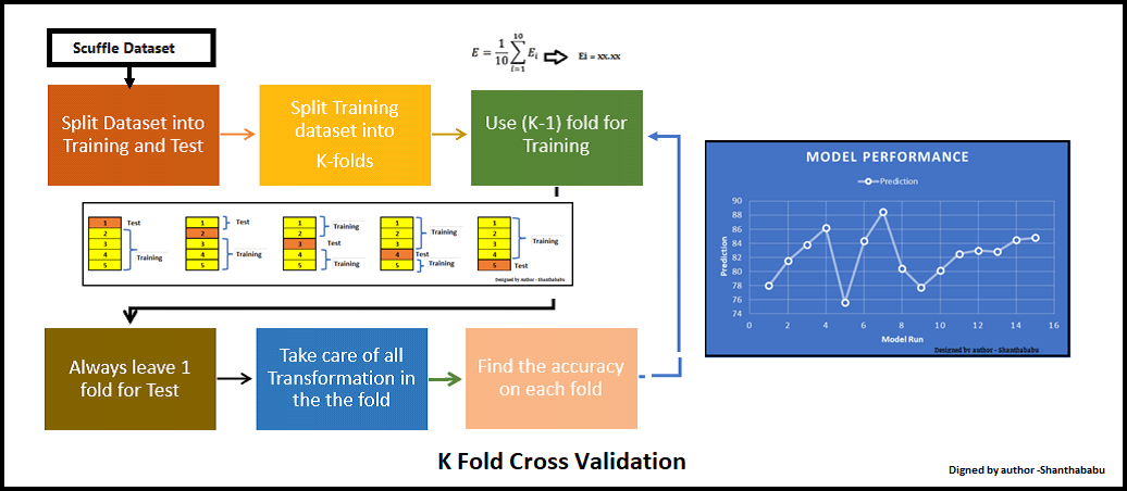
Validation sets and cross-validation are crucial tools for model assessment and hyperparameter tuning in supervised learning.

• A validation set acts as an intermediate checkpoint during model training.

• It's a portion, typically 20-30%, of the original dataset (training set).

• After initial training on the training set, the model is evaluated on the validation set to gauge its performance.

• This provides insights into how the model might perform on new, unseen data.

• If a model performs extremely well on the training set but poorly on the validation set, it's likely overfit.

• Overfitting happens when a model becomes too attuned to random quirks or noise in the training data, making it less effective on new data.

• Utilizing the validation set, you can recognize overfitting and employ strategies like data augmentation, feature selection, or regularization to manage it.

• Cross-validation (CV) takes the concept of a validation set a step further by using the entire dataset for both training and validation in a systematic way.

• It overcomes the randomness that can arise from a single validation set by using multiple non-overlapping subsets of the data, called folds.

• The most common form of CV is k-fold, where the original dataset is partitioned into k equal-sized folds. The model is trained and evaluated k times, each time using a different fold for validation.

• Each partition serves as a validation set, while the remaining data is used for training.

• The final performance metric is the average of the metrics obtained from k iterations.

• Optimal Data Utilization: Every data point is utilized for both training and validation, which is particularly useful when the dataset is limited.

• Robustness: By averaging multiple performance scores, we get a more reliable estimate of model performance, reducing the impact of randomness or quirks present in a single dataset partition.

• Hyperparameter Optimization: It helps in selecting the most suitable set of hyperparameters for the model.

• Stratified Cross-Validation: A variation suitable for imbalanced datasets where each fold ensures a similar class distribution as the original.

• Leave-One-Out Cross-Validation (LOOCV): Particularly useful for smaller datasets, where one data point is left out for validation, and the rest are used for training.

• Time Series Cross-Validation: Suited for time-dependent data, ensuring validation on future time points.

Regularization is a set of techniques used to prevent overfitting in machine learning models, especially in Supervised Learning. Overfitting occurs when a model learns training data too well, to the extent that it performs poorly on unseen data.

Regularization helps strike a balance between capturing intricate patterns in the training data and generalizing well to new data. Without regularization, complex models can memorize even random noise in the training data, leading to overfitting.

• L1 Regularization (LASSO): Introduces a penalty proportional to the absolute value of the model's coefficients. This can cause some coefficients to become zero, effectively performing feature selection.

• L2 Regularization (Ridge): Adds a penalty proportional to the square of the coefficients, leading to smaller coefficient values.

• Elastic Net: Combines L1 and L2 penalties, providing a balance between feature selection and coefficient size reduction.

• Data Augmentation: For computer vision tasks, data is augmented by performing various transformations like rotation, flipping and cropping on the training data.

• Dropout: Used in neural networks, where during training, a random set of neurons are dropped (i.e., their output is set to zero) in each iteration.

• Early Stopping: The training process is halted when model performance on a validation set stops improving, thus preventing the model from learning noise in the training data.

• Bagging and Boosting: These techniques work by training models on different subsets of data and then combining their outputs, effectively regularizing the model.

• Max Norm Constraint: In this technique, the L2-norm of model weights is constrained to a certain threshold.

• Batch Normalization: This technique involves normalizing the output of each layer, reducing the likelihood of overfitting.

• Unsupervised Pre-training: This method involves training individual layers or components of the model in an unsupervised manner before fine-tuning the entire model using supervised learning.

• Multi-Task Learning: This type of learning involves training a single model on multiple related tasks, which can help improve the model's generalization.

Many of these techniques are inter-related and can be used in tandem for more effective regularization.

Linear Regression is one of the simplest and most fundamental supervised learning algorithms. It's widely used for both regression and predictive analysis.

• Line of Best Fit: It finds the best-fitting linear relationship between independent variables (features) and a target variable.

• Objective Function: Linear regression aims to minimize the difference between actual and predicted values by optimizing an objective function, often the mean squared error.

• Input Data: Pairs of input (independent) variables $(x_1, x_2, \ldots, x_n)$ and the output (dependent) variable $y$.

• Model: Visualized as a line, mathematically represented as $y = mx + c$.

• Coefficients: $m$ (slope) and $c$ (intercept) are determined to define the line that best fits the data.

• Training: Achieved by estimating the coefficients that minimize the objective function. This process is referred to as "fitting the model."

• Testing and Validation: Model accuracy is assessed using test datasets. Common metrics include Mean Absolute Error, Mean Squared Error, and Root Mean Square Error.

Linear regression assumes a linear relationship between the input features and output. It aims to find the line that minimizes the squared differences between observed and predicted values.

The model predicts the target variable $y$ as a linear combination of input features $X$ and coefficients $W$, plus an error term $e$:

$$ y = X \cdot W + e $$

The objective function to minimize during training is often the Mean Squared Error (MSE):

$$ MSE = \frac{1}{n}\sum_{i=1}^{n} (y_i - \hat{y}_i)^2 $$

Where:

• $n$ is the number of data points.
• $y_i$ and $\hat{y}_i$ are the true and predicted target values, respectively.

The most common approach, OLS, uses matrix operations to calculate the coefficients that minimize the squared error. It directly computes optimal $W$ values as:

$$ W = (X^T X)^{-1} X^T y $$

Where:

• $X$ is the input feature matrix (with each row representing a data point, and each column a feature).
• $y$ is the target variable vector.
• $^T$ denotes the matrix transpose.
• $^{-1}$ represents the matrix inverse operation.

Linear regression is often used in scenarios where the relationship between independent and dependent variables is linear. It serves as a baseline model in many applications like:

• Identifying relationships between consumer behaviour and marketing outreach.
• Financial modeling to predict stock prices or economic indicators.
• Resource allocation in areas such as healthcare and education.

When data doesn't exhibit a strictly linear trend, polynomial regression can be applied to fit non-linear relationships.

To combat issues like overfitting, techniques like Ridge, Lasso, and Elastic Net use regularization, adding a penalty term to the objective function.

Accounting for the presence of outliers, robust regression methods are less sensitive to these data points.

Despite its name, logistic regression is a classification algorithm that's closely related to linear regression. Instead of predicting a continuous value, it outputs the probability of belonging to a particular class.

Linear Regression serves as the foundation for numerous advanced regression techniques, making it a prevalent tool in machine learning and statistics.

• Definition: A straightforward approach best suited for scenarios where one predictor variable ($x$) impacts one target variable ($y$).

• Equation:

$$ y = \beta_0 + \beta_1x + \epsilon $$

where $\epsilon$ captures the error term.

• Visual Representation: This method visualizes relationships with a single $x$-$y$ scatter plot.

• Model Complexity: Has one slope and one intercept.

• Definition: A highly adaptable technique where multiple predictor variables influence a single target. Distinguished by its flexibility, it's capable of handling diverse datasets. The equation is mathematically more generalized and works on N-dimensions.

• Equation in Vector Notation:

$$ Y = X\beta + \epsilon $$

or in component form:

$$ Y_i = \beta_0 + \sum_{j=1}^{p}\beta_jx_{ij} + \epsilon_i $$

• Visual Representation: The method visualizes individual relationships using matrices like scatter plots and correlation matrices.

• Model Complexity: The equation is characterized by multiple slopes and a single intercept.

• Complexity: SLR predicts the response based on one input variable, while MLR uses multiple predictors.

• Mathematical Representation: The equation for SLR is straightforward, whereas MLR uses matrix notation.

• Matrix Notation: In MLR, the independent variables (features or attributes) are represented as a matrix, $X$, while the coefficients are a vector, $\beta$.

• Interpretation: In SLR, the slope quantifies the magnitude of the change. In MLR, partial slopes show the isolated effects of each predictor while keeping others constant.

• Residual Analysis: While both SLR and MLR employ residual diagnostics, MLR allows for a deeper diagnostic through the study of Partial Residual Plots. These plots show the relationship between a predictor and the response, adjusted for the effects of other predictors.

• Use of the F-test: While SLR typically uses a t-test, MLR can take advantage of the additional F-test to assess the significance of the model as a whole and the collective effect of all predictors.

Logistic Regression is a statistical method widely used for binary classification and probability estimation.

• Predicted Variable: Binary (0/1, True/False, Yes/No)
• Input Variables: Numerical or categorical
• Model Type: Probabilistic
• Main Algorithm: Maximum Likelihood Estimation

The algorithm transforms the output of a linear equation, $z = w_1x_1 + w_2x_2 + \ldots + b$, using a logistic or sigmoid function:

$$ \sigma(z) = \frac{1}{1 + e^{-z}} $$

This leads to a non-linear 'S'-shaped probability curve, providing the predicted probability $\hat{y}$ as the output.

The probability curve intersects the vertical line at $z = 0$ where $\sigma(z) = 0.5$. Mathematically:

$$ $$ \sigma(z) & = 0.5 \\ \frac{1}{1 + e^{-z}} & = 0.5 \\ 1 + e^{-z_0} & = 2 \\ e^{-z_0} & = 1 \\ -z_0 & = 0 \\ z_0 & = 0 $$ $$

Hence, the decision boundary in feature space $x$ is linear.

In Logistic Regression, the goal is to learn the optimal weights $w$ and the bias term $b$. Standard optimization techniques like Gradient Descent or L-BFGS minimize a loss function, often the Cross-Entropy Loss.

1. Healthcare: Disease prediction based on symptoms and patient history.
2. Marketing: Customer response prediction to campaigns.
3. Finance: Credit scoring and loan default prediction.
4. Natural Language Processing (NLP): Text sentiment analysis.
5. Image Recognition: Object detection and image classification.

Here is the Python code:

from sklearn.linear_model import LogisticRegression
from sklearn.model_selection import train_test_split
from sklearn.metrics import accuracy_score, classification_report
import pandas as pd

# Load your dataset
data = pd.read_csv('your_dataset.csv')

# Split into features and target
X = data.drop('target_variable', axis=1)
y = data['target_variable']

# Train/Test Split
X_train, X_test, y_train, y_test = train_test_split(X, y, test_size=0.2, random_state=42)

# Instantiate the model
model = LogisticRegression()

# Train the model
model.fit(X_train, y_train)

# Predictions
y_pred = model.predict(X_test)

# Model evaluation
print(f"Accuracy: {accuracy_score(y_test, y_pred)}")
print(classification_report(y_test, y_pred))

In a nutshell, Ridge Regression uses a regularization term called the L2 penalty to prevent overfitting. The penalty term constrains the model from becoming too complex, thus enhancing its generalization ability.

Ridge Regression, also known as L2 Regularization, uses the following loss function:

$$ LossRSS+W|\beta|^2 $$

where:

• $LossRSS$ is the Residual Sum of Squares (RSS)
• $W$ is the regularization parameter
• $|\beta|^2$ represents the squared L2 norm of the coefficient vector, $\beta$

As the value of $W$ increases, the penalty term becomes more dominant, leading to shrinkage of the coefficients.

The ridge coefficients are the values that minimize the combined loss of the RSS and the L2 penalty. They can be derived via the formula:

$$ \hat{\beta}^{ridge} = (X^TX + \lambda I)^{-1}X^Ty $$

Where:

• $X$ is the design matrix
• $y$ is the target vector
• $\lambda$ is the regularization parameter
• $I$ is an identity matrix

Notice that the term $X^TX$ has the effect of scaling the coefficients. The addition of $\lambda I$ introduces *ridge that improves stability and generalization.

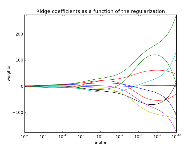
In the plot, "Ridge" accentuates how coefficient values deviate from zero as $\lambda$ increases.

Here is the Python code:

from sklearn.linear_model import Ridge
import numpy as np

# Simulated data
X = np.array([[1, 1], [1, 2], [2, 2], [2, 3]])
y = np.array([1, 2, 3, 4])

# Fitting the Ridge Regression model
ridge = Ridge(alpha=1.0)
ridge.fit(X, y)

# Accessing the coefficients
print(ridge.coef_)

LASSO Regression (Least Absolute Shrinkage and Selection Operator) is a regularization technique that optimizes the coefficients' values in a linear regression model while introducing a penalty to reduce overfitting.

Lasso Regression is distinctive for its property of variable selection.

The cost function for Lasso Regression is a combination of the least squares' error term and the L1-norm of the coefficients (which represents the absolute values of the coefficients):

$$\text{Cost} = \text{SSE} + \lambda \sum_{i=1}^{n}|{\beta}_i|$$

• SSE: Sum of Squared Errors
• $\beta_i$: Model coefficient for the $i$-th feature
• $n$: Total number of features
• $\lambda$: Regularization parameter that controls the shrinkage strength

As the L1-norm of the coefficients is minimized, many coefficients may become exactly zero, leading to a sparse model that performs feature selection.

• In a marketing context, Lasso Regression can help identify key variables for customer conversion.
• In genetics and bioinformatics, Lasso Regression aids in identifying significant genetic markers related to specific traits or diseases.
• In scientific research, Lasso can help select the most influential independent variables when studying complex systems, such as climate models.

Here is the Python code:

from sklearn.datasets import load_boston
from sklearn.linear_model import Lasso
from sklearn.model_selection import train_test_split
from sklearn.preprocessing import StandardScaler
from sklearn.metrics import mean_squared_error
import numpy as np

# Load data
boston = load_boston()
X, y = boston.data, boston.target
feature_names = boston.feature_names

# Split data
X_train, X_test, y_train, y_test = train_test_split(X, y, test_size=0.25, random_state=42)

# Standarize features
scaler = StandardScaler()
X_train = scaler.fit_transform(X_train)
X_test = scaler.transform(X_test)

# Fit Lasso model
lasso = Lasso(alpha=0.1)  # Here, alpha is the regularization parameter (lambda)
lasso.fit(X_train, y_train)

# Print coefficients
coef_names = list(zip(feature_names, lasso.coef_))
print("Lasso Coefficients:\n", coef_names)

# Evaluate model
y_pred = lasso.predict(X_test)
mse = mean_squared_error(y_test, y_pred)
print("Mean Squared Error (MSE):", mse)