Random Forest is an ensemble learning method based on decision trees. It operates by constructing multiple decision trees during the training phase and outputs the mode of the classes or the mean prediction of the individual trees.

1. Decision Trees: Basic building blocks that segment the feature space into discrete regions.

2. Bootstrapping (Random Sampling with Replacement): Each tree is trained on a subset of the data, enabling robustness and variance reduction.

3. Feature Randomness: By considering only a subset of features, diversity among the trees is ensured. This is known as attribute bagging or feature bagging.

4. Voting or Averaging: Predictions from individual trees are combined using either majority voting (in classification) or averaging (in regression) to produce the ensemble prediction.

• Bootstrapping: Each tree is trained on a different subset of the data, improving diversity and reducing overfitting.

• Feature Randomness: A random subset of features is considered for splitting in each tree. This approach helps to mitigate the impact of strong, redundant, or irrelevant features while promoting diversity.

• Majority Vote: In classification, the most frequently occurring class label is the predicted class for a new instance, as determined by the individual trees.

• Quick Training: Compared to certain other models, Random Forests are relatively quick to train even on large datasets, making them suitable for real-time applications.

• Node Splitting: The selection of the optimal feature for splitting at each node is guided by feature importance measures such as Gini impurity and information gain.

• Stopping Criteria: Trees stop growing when certain conditions are met, such as reaching a maximum depth or when nodes contain a minimum number of samples.

• Ensemble Prediction: All trees "vote" on the outcome, and the class with the most votes is selected (or the mean in regression).

• Out-of-Bag Estimation: Since each tree is trained on a unique subset of the data, the remaining, unseen portion can be used to assess performance without the need for a separate validation set.

  This is called out-of-bag (OOB) estimation. The accuracy of OOB predictions can be averaged across all trees to provide a robust performance measure.

• Cross-Validation: Techniques like k-fold cross-validation can help identify the best parameters for the Random Forest model.

• Hyperparameters: Key parameters to optimize include the number of trees, the maximum depth of each tree, and the minimum number of samples required to split a node.

Here is the Python code:

from sklearn.ensemble import RandomForestClassifier
from sklearn.datasets import load_iris
from sklearn.model_selection import train_test_split
from sklearn.metrics import accuracy_score

# Load the Iris dataset
iris = load_iris()
X, y = iris.data, iris.target

# Split the data into training and testing sets
X_train, X_test, y_train, y_test = train_test_split(X, y, test_size=0.3, random_state=42)

# Instantiate the random forest classifier
rf = RandomForestClassifier(n_estimators=100, random_state=42)

# Train the model
rf.fit(X_train, y_train)

# Make predictions on the test data
predictions = rf.predict(X_test)

# Assess accuracy
accuracy = accuracy_score(y_test, predictions)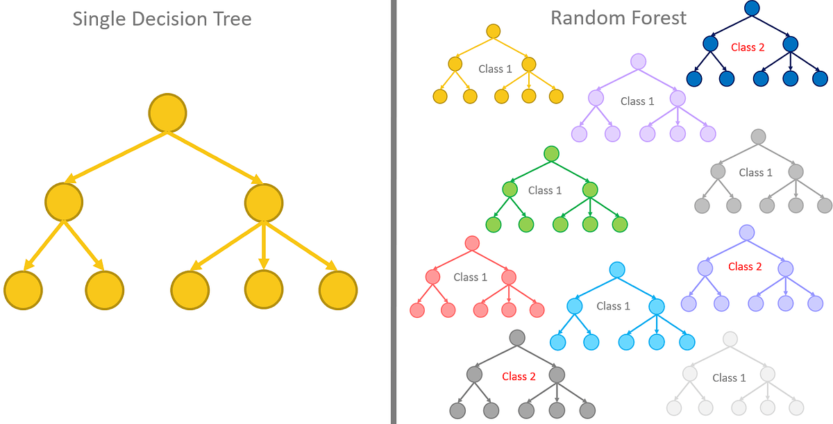
print(f"Accuracy: {accuracy*100:.2f}%")

Let's explore the key differences between a Random Forest (RF) model and a single decision tree (DT algorithm). This will give us insights into the strengths and weaknesses of each approach.

A Random Forest is an ensemble learning method that combines the predictions of multiple decision trees. Each tree in the forest is trained on a randomly sampled subset of the training data and uses a random subset of features at each split point, hence the name.

1. Accuracy: On average, a Random Forest generally outperforms a single decision tree. This is because the Random Forest is less prone to overfitting, given the process of bootstrapping and feature selection.

2. Robustness: Since a Random Forest is an ensemble of trees, its overall performance is more reliable and less susceptible to noise in the data.

3. Optimization: Tuning a single decision tree can be quite complex, but Random Forests are less sensitive to hyperparameter settings and hence are easier to optimize.

4. Feature Importance: Random Forests provide a more reliable method for determining feature importance, as it's averaged over all trees in the ensemble.

5. Handling Missing Data: The algorithm can handle missing values in predictors, making it more versatile.

6. Parallelism: Individual trees in a Random Forest can be trained in parallel, leading to faster overall training compared to a single decision tree.

1. Model Interpretability: Random Forests are not as straightforward to interpret as a single decision tree, which can be visualized and easily understood.

2. Resource Consumption: Random Forests typically require more computational resources, especially when the dataset is large.

3. Prediction Time: Making real-time predictions can be slower with Random Forests, especially when compared to a single decision tree.

4. Disk Space: Saving a trained Random Forest model can require more disk space when compared to a single decision tree due to the many trees in the ensemble.

Random Forests offer several advantages:

• Robustness: They handle well both noisy data and overfitting issues.

• Feature Importance: The forest's construction allows for easy ranking of feature importance.

• Scalability: The ensemble learning structure of Random Forests makes them naturally fit for parallelizing tasks. This means the model can scale with a larger dataset.

• Convenience: Random Forests don't usually require extensive data preparation or fine-tuning of hyperparameters.

• Flexibility: They can perform well on both classification and regression tasks.

• Handles Missing Data: The decision tree algorithm at the core of Random Forests can handle missing values, which means you may not always need to preprocess your data.

• Balanced Datasets: Random Forests can handle imbalanced datasets without the need for specific techniques, like re-sampling.

• Insensitivity to Outliers: The nature of the algorithm makes Random Forests less affected by outliers. This can be an advantage or disadvantage, depending on the use case.

• Suitability for Mixed Datasets: They can effectively handle datasets with both numerical and categorical data.

Bagging, short for boostrap aggregating, is a technique that leverages ensemble methods to boost predictive accuracy. It achieves this by training multiple models using various subsets of the dataset and then combining their predictions. The two primary components of bagging are bootstrapping and aggregation.

This method involves repeatedly sampling the dataset with replacement, resulting in several training datasets of the same size as the original but with varied observations. Bootstrapping enables the construction of diverse models, enhancing the ensemble's overall performance.

Bagging employs averaging for regression tasks and majority voting for classification tasks to aggregate the predictions made by each model in the ensemble.

1. Data Division: A Random Forest partitions the dataset into distinct subsets called decision trees. Each tree in the forest is built using a different bootstrapped sample.

2. Training the Trees: Both feature selection and bootstrapping are involved in training each decision tree. During the bootstrapping process, every tree is constructed with a subset of data sampled with replacement. Feature selection is done at each split, and the available features are a random subset of the full feature set. This randomization ensures the diversity of the individual trees.

3. Prediction Aggregation: For regression tasks, random forests aggregate predictions by averaging them, while for classification tasks, they use majority voting. Each tree's prediction is considered, and the combined final prediction is made based on the aggregation method.

4. Importance: Random Forests calculate the feature importance through a mechanism known as mean decrease in impurity, which quantifies how each feature contributes to the predictive accuracy of the forest.

Bagging can be seen as a method to reduce variance. By training multiple models on various bootstrapped samples and then averaging their predictions, the hope is that the overall prediction error will be lower, leading to better generalization on unseen data.

The intuition behind this approach is that, while individual models may overfit to their particular training set, combining their predictions reduces the risk of overfitting. This reduction in overfitting leads to a decrease in variance.

The bagging method, as encapsulated by random forests, typically excels in reducing overfitting and enhancing accuracy.

While the individual trees in a random forest might not be as interpretable or precise as some other models, their combined strength often results in highly accurate predictions.

Here is the Python code:

from sklearn.ensemble import RandomForestClassifier
from sklearn.model_selection import train_test_split
from sklearn.datasets import load_iris
from sklearn.metrics import accuracy_score

# Load dataset
iris = load_iris()
X, y = iris.data, iris.target

# Split data
X_train, X_test, y_train, y_test = train_test_split(X, y, test_size=0.2, random_state=42)

# Initialize the Random Forest classifier
clf = RandomForestClassifier(n_estimators=100, random_state=42)

# Fit the model to the training data
clf.fit(X_train, y_train)

# Make predictions
y_pred = clf.predict(X_test)

# Assess accuracy
accuracy = accuracy_score(y_test, y_pred)
print(f"Accuracy: {accuracy:.4f}")

Random Forest achieves feature randomness through a process called bootstrap aggregating or bagging. For feature selection, each tree is trained on a subset of the original feature set, promoting both diversity and robustness.

1. Bootstrap Sampling: A random subset of the training data is repeatedly sampled with replacement. This leads to different subsets for each tree, ensuring diversity.

2. Feature Subset Selection: A hyperparameter, often referred to as "max_features", is predefined. It specifies the maximum number of features allowed.

3. Tree Construction: Each decision tree is built on its unique bootstrap sample and feature subset.

4. Voting Mechanism: For prediction, individual tree outputs are combined by majority vote (for classification) or averaging (for regression).

Here is the Python code:

from sklearn.ensemble import RandomForestClassifier
from sklearn.datasets import make_classification
from sklearn.model_selection import train_test_split

# Generate sample data
X, y = make_classification(n_samples=1000, n_features=20, random_state=42)

# Split the data into training and test sets
X_train, X_test, y_train, y_test = train_test_split(X, y, test_size=0.2, random_state=42)

# Define and fit the random forest classifier
rf_clf = RandomForestClassifier(n_estimators=100, max_features="sqrt", random_state=42)
rf_clf.fit(X_train, y_train)

# Get feature importances
feature_importances = rf_clf.feature_importances_
print(feature_importances)

In this example, by setting max_features to "sqrt", feature randomness is incorporated based on each tree's square root of the total features.

• Regularization: By excluding non-informative features and reducing correlations among trees, random forest becomes less prone to overfitting. This enhancement is especially useful when dealing with high-dimensional datasets.
• Enhanced Diversity: Inputting fewer features in each tree increases the variability among the trees in the forest, leading to more diverse models.
• Improved Interpretability: Focusing on distinct sets of predictors across trees can aid in understanding feature importance and selection.

In Random Forest models, the out-of-bag (OOB) error is a metric that gauges the classifier's accuracy using data that was not part of the bootstrapped sample for training.

1. Bootstrapped Sample: Each tree in a Random Forest is trained on a subset of the total data, created through bootstrapping: random sampling with replacement. Consequently, not all data points are used for training in every tree.

2. Majority Vote: Ensemble Aggregation: For each data point not present in a tree's bootstrapped sample, the corresponding tree contributes to a majority vote. The most common class among all trees for that data point is then assigned as the final prediction.

3. Error Computation: By comparing the OOB-derived predictions to the actual known class labels, an error rate is calculated. This is then averaged across all data points not used in a particular tree's training.

• Proximity to CV-based Error: In small to medium datasets, the OOB error rate approximates the performance of the test dataset from k-fold cross-validation.

• No Need for Dedicated Test Sets: The OOB error provides a noisier but still valuable estimate of the model's performance, removing the need for a separate test set in smaller datasets or during model development.

• Real-Time Performance Monitoring: As Random Forests are robust to overfitting, the OOB error facilitates continuous model assessment during training. However, for a more definitive assessment of performance, a dedicated test set should still be used, especially in large datasets.

Random Forests, unlike certain other algorithms, are not unduly influenced by attributes with more levels or categories.

Bagging, the base technique for Random Forest, thrives on diversity among individual trees.

1. Each tree is trained on a bootstrapped sample, i.e., only a subset of the dataset. This promotes variation, reducing potential bias toward attributes with more levels.

2. For each node in every tree, only a subset of attributes is considered for the best split. This randomly selected subset diminishes the impact of any single attribute, balancing their influences.

• Feature Engineering: Construct attributes to be as meaningful as possible, no matter the number of levels.
• Exploratory Data Analysis (EDA): Understand the dataset thoroughly to make informed decisions about its attributes.
• Data Preparation: Scaling, encoding, and handling missing values are crucial steps that can significantly affect the model's outcome.

A Random Forest model handles missing data effectively during both training and test stages. It does so through sophisticated methods such as proximity measures and imputation.

During the bootstrapping process in RF training, missing values in features are addressed by using a method called "Out-of-Bag (OOB)".

The Gini index or entropy reduction, for example, is calculated for decision trees based on observed features in a subset of the data.

When making predictions during testing, RF models can adapt to missing data through techniques such as averaging or voting based on the available features.

Here is the Python code:

# Data Preparation
from sklearn.model_selection import train_test_split
import numpy as np

X = np.array([[1, 2], [np.nan, 3], [7, 6], [3, 4], [np.nan, 5]])
y = np.array([0, 1, 2, 3, 4])

X_train, X_test, y_train, y_test = train_test_split(X, y, test_size=0.2)

# Import and Initialize Random Forest
from sklearn.ensemble import RandomForestClassifier
clf = RandomForestClassifier()

# Model Fitting
clf.fit(X_train, y_train)

# Predictions - These will handle missing values
prediction = clf.predict(X_test)

Random Forest, a robust ensemble learning method, is built upon a collection of decision trees. The accuracy and generalizability of the forest hinges on specific hyperparameters.

1. n_estimators

   • Number of trees in the forest.
   • Effect: Higher values can lead to improved performance, although they also increase computational load.
   • Typical Range: 100-500.

2. max_features

   • Maximum number of features considered for splitting a node.
   • Effect: Controlling this can mitigate overfitting.
   • Typical Values: "auto" (square root of total features), "sqrt" (same as "auto"), "log2" (log base 2 of total features), or specific integer/float values.

3. max_depth

   • Maximum tree depth.
   • Effect: Regulates model complexity to combat overfitting.
   • Typical Range: 10-100.

4. min_samples_split

   • Minimum number of samples required to split an internal node.
   • Effect: Influences tree depth and a smaller value may lead to overfitting.
   • Typical Values: 2-10 for a balanced dataset.

5. min_samples_leaf

   • Minimum number of samples required to be at a leaf node.
   • Effect: Helps smooth predictions and can deter overfitting.
   • Typical Values: 1-5.

6. bootstrap

   • Indicates whether to use the bootstrap sampling method.
   • Effect: Setting it to "False" obstructs bootstrapping and can diversity in the models.
   • Typical Value: "True".

While machine learning models have default hyperparameter values, such as n_estimators=100, it is crucial to fine-tune these parameters to optimize a model for a specific task. This process is known as hyperparameter tuning. A common technique for hyperparameter tuning is to use grid search, which systematically searches through a grid of hyperparameter values to find the best model.

Here is the Python code:

from sklearn.ensemble import RandomForestClassifier
from sklearn.model_selection import GridSearchCV

# Create a random forest classifier
rf = RandomForestClassifier()

# Define the grid of hyperparameters to search
param_grid = {
    'n_estimators': [100, 200, 300],
    'max_depth': [10, 20, 30, 40, 50, None],
    'min_samples_split': [2, 5, 10],
    'min_samples_leaf': [1, 2, 4],
    'bootstrap': [True, False]
}

# Perform grid search with defined grid and cross-validation
grid_search = GridSearchCV(estimator=rf, param_grid=param_grid, cv=5, n_jobs=-1)
grid_search.fit(X_train, y_train)

# Get the best hyperparameters
best_params = grid_search.best_params_
print(best_params)

Random Forest is a versatile supervised learning algorithm that excels in both classification and regression tasks. Its adaptability and performance in diverse domains make it a popular choice in the ML community.

A Random Forest employs an ensemble of decision trees to make discrete predictions across multiple classes or categories. Each tree in the forest independently "votes" on the class label, and the most popular class emerges as the final prediction.

Contrary to dividing data into classes, the Random Forest algorithm serves up continuous predictions in a regression task. Trees in the forest predict numerical values, and the final outcome is often determined by averaging these values.

Many modern libraries, such as scikit-learn, have streamlined the process, unifying classification and regression under a single method, predict. This unification further simplifies model implementation and reduces the possibility of errors.

Here is the Python code:

# Import the Random Forest model
from sklearn.ensemble import RandomForestClassifier, RandomForestRegressor

# Example dataset
X = [[0, 0], [0, 1], [1, 0], [1, 1]]
Y_classification = [0, 1, 1, 0]
Y_regression = [0, 1, 2, 3]

# Instantiate the models
rfc = RandomForestClassifier()
rfr = RandomForestRegressor()

# Train the models
rfc.fit(X, Y_classification)
rfr.fit(X, Y_regression)

# Make unified predictions
print("Unified Classification Prediction:", rfc.predict([[0.8, 0.6]])[0])
print("Unified Regression Prediction:", rfr.predict([[0.9, 0.9]])[0])

Ensemble Learning combines the predictions of multiple models to improve accuracy and robustness. Random Forest is an ensemble of Decision Trees, and its distinct construction and operational methods contribute to its effectiveness.

Ensemble methods aggregate predictions from multiple individual models to yield a final, often improved, prediction. This approach is based on the concept that diverse models, or models trained on different subsets of the data, are likely to make different errors. Through combination, these errors may cancel each other out, leading to a more accurate overall prediction.

• Forest Formation: A Random Forest comprises an ensemble of Decision Trees, each trained independently on a bootstrapped subset of the data. This process, known as bagging, promotes diversity by introducing variability in the training data.

• Feature Subset Selection: At each split in the tree, the algorithm considers only a random subset of features. This mechanism, termed feature bagging or random subspace method, further enhances diversity and protects against overfitting.

• Majority Voting: For classification tasks, the mode (most common class prediction) of the individual tree predictions is taken as the final forest prediction. In the case of regression tasks, the average of the individual tree predictions is computed.

1. Bootstrapped Data: Random Forest selects $n$ samples with replacement from the original dataset to form the training set for each tree.

2. Feature Subspace Sampling: On account of feature bagging, a random subset of $m$ features is chosen for each split in the tree. The value of $m$ can be set by the user or is automatically determined through tuning.

3. Decision Tree Training: Each Decision Tree is trained on the bootstrapped dataset using one of several techniques, such as CART (Classification and Regression Trees).

4. Aggregation: For classification, the mode is determined across the predictions of all the trees. For regression, the average prediction across trees is taken.

• Robustness: By aggregating predictions across multiple trees, Random Forest is more robust than individual Decision Trees.
• Decreased Overfitting: Through bootstrapping and feature bagging, the risk of overfitting is mitigated.
• Computational Efficiency: The parallelized nature of tree construction in Random Forest can lead to computational efficiencies in multi-core environments.

• Lack of Transparency: The combined decision-making can make it harder to interpret or explain the model's predictions.
• Potential for Overfitting: In certain cases or with certain parameter settings, Random Forest models can still overfit the training data.
• Feature Importance: The feature importances provided by Random Forest can be biased in the presence of correlated features.
• Hyperparameter Tuning: Although Random Forest models are less sensitive to hyperparameters, it's still important to tune them for optimal performance.

Here is the Python code:

from sklearn.ensemble import RandomForestClassifier
from sklearn.datasets import make_classification
from sklearn.model_selection import train_test_split
from sklearn.metrics import accuracy_score

# Create a random forest classifier
X, y = make_classification(n_samples=1000, n_features=20, random_state=42)
X_train, X_test, y_train, y_test = train_test_split(X, y, test_size=0.2, random_state=42)
rf_classifier = RandomForestClassifier(n_estimators=100, random_state=42)

# Train the classifier
rf_classifier.fit(X_train, y_train)

# Make predictions on the test data
y_pred = rf_classifier.predict(X_test)

# Calculate accuracy
accuracy = accuracy_score(y_test, y_pred)
print(f"Random Forest Accuracy: {accuracy}")

Both Random Forest (RF) and Gradient Boosting Machine (GBM) are popular ensemble methods, but they achieve this through different mechanisms.

• Ensemble Approach: Both RF and GBM are ensemble methods that combine the output of multiple individual models. This generally results in more accurate, robust, and stable predictions compared to a single model.

• Decision Trees as Base Learners: Both methods often use decision trees as base learners for their individual models. These decision trees are honed, either independently or in sequence, to make predictions.

• Tree Parameters: Both RF and GBM offer means to control individual tree complexity, such as maximum depth, minimum samples per leaf, and others. These parameters assist in avoiding overfitting, which can be a common issue with decision trees.

• RF: Decision-making across trees is made independently, and the majority vote determines the final prediction.
• GBM: Trees are constructed sequentially, and each new tree focuses on reducing the errors made by the ensemble up to that point.

• RF: Uses bootstrapping to randomly sample data, which means each tree is built on a different subset of the training data. These trees are then aggregated in a parallel fashion.
• GBM: Utilizes all available data for building trees but assigns different weights to the data points to adjust the focus on certain regions over time.

• RF: The final prediction is made by majority voting across all the trees.
• GBM: Final prediction is attained by summing the predictions of each sequential tree, often combined with a learning rate.

• RF: Due to its inherent mechanism of building and evaluating each tree, RF is less prone to overfitting on the dominant class, leading to better performance on imbalanced datasets.
• GBM: It's sometimes sensitive to class imbalance, making it crucial to set appropriate hyperparameters.

• RF: While simpler to understand and implement, RF can be less sensitive to changes in its parameters, especially when the number of trees is high. This can make fine-tuning more challenging.
• GBM: The sequential nature of GBM makes it more tunable and sensitive to individual tree and boosting parameters, lending itself to optimization via methods like cross-validation.

• RF: Inherently parallel, RF denotes an attractive choice for large datasets and effortless distribution over multiprocessing units.
• GBM: Typically implemented in a sequential manner, but "Gradient Boosting" libraries often provide options, like histogram-based techniques, for parallelized execution.

• RF: Feature importance is computed based on the individual information gain of the trees built on the training data.
• GBM: It calculates feature importance on the basis of how important each feature was for reducing the errors in the predictions made by the ensemble.

• Adaptive Learning: GBM adapts its learning strategy to prioritize areas where it hasn't performed well in the past, making it effective in regions where the data is challenging.
• Sensitivity to Noisy Data: GBM could overfit on noisy data, mandating careful treatment of such data points.

• Versatile and Less Sensitive to Hyperparameters: Random Forest can perform robustly with less tuning, making it an excellent choice, particularly for beginners.
• Efficiency with Larger Feature Sets: RF can handle datasets with numerous features and still perform efficiently in terms of training time.

While both Random Forest (RF) and Extra Trees (ET) classifiers belong to the ensemble of decision trees, they each have unique characteristics that make them suited to specific types of datasets.

1. Decision Process:

   • RF: Uses a bootstrapped sample and a feature subset to build multiple trees.
   • ET: Constructs each tree using the entire dataset and a randomized feature selection.

2. Node Splitting:

   • RF: Employs a best split as determined by Gini impurity or information gain.
   • ET: Chooses random splits, gaining efficiency at the cost of potential accuracy.

3. Bagging vs. Bootstrapping:

   • RF ('Bagging'): Resamples from the dataset to train different trees.
   • ET ('Pasting'): Trains each tree with the complete dataset.

4. Performance Guarantee:

   • RF: Steady, yet possibly less predictive.
   • ET: Faster, but with an occasional sacrifice in predictive accuracy.

5. Variability in Trees:

   • RF: Each tree is trained using bootstrapped replicas of the dataset, resulting in some level of correlation between trees.
   • ET: Each tree is trained using the entire dataset, potentially resulting in less diverse trees.

6. Feature Subset Selection:

   • RF: Employs a subset of features for each node.
   • ET: Utilizes the complete feature set.

7. Hyperparameter Sensitivity:

   • RF: Slightly less sensitive due to feature subsampling.
   • ET: Sensitive due to apparent lack of stabilization mechanisms.

Random Forest employs several decision trees constructed on bootstrapped datasets with an added layer of randomness to increase robustness and mitigate overfitting, offering features distinct from traditional Decision Trees.

• Bootstrap Aggregating (Bagging):

  • Each tree is built on a unique subset of the training data, selected with replacement.
  • Subsampling reduces the impact of noisy or outlier data.

• Variable Randomness:

  • At each split, a random subset of features is considered. This mechanism counteracts the preference of Decision Trees to select the most discriminative features.

• Ensemble Averaging:

  • Output is the average prediction of all trees, rather than a majority vote. This helps mitigate overfitting, particularly in regression tasks.

Here is the Python code:

from sklearn.ensemble import RandomForestClassifier
from sklearn.tree import DecisionTreeClassifier
from sklearn.model_selection import train_test_split
from sklearn.datasets import load_iris
from sklearn.metrics import accuracy_score

# Load the Iris dataset
iris = load_iris()
X, y = iris.data, iris.target
X_train, X_test, y_train, y_test = train_test_split(X, y, test_size=0.33, random_state=42)

# Train Decision Tree and Random Forest models
dt = DecisionTreeClassifier(random_state=42)
dt.fit(X_train, y_train)

rf = RandomForestClassifier(n_estimators=100, random_state=42)
rf.fit(X_train, y_train)

# Evaluate models
dt_pred = dt.predict(X_test)
rf_pred = rf.predict(X_test)

dt_accuracy = accuracy_score(y_test, dt_pred)
rf_accuracy = accuracy_score(y_test, rf_pred)

print(f'Decision Tree Accuracy: {dt_accuracy}')
print(f'Random Forest Accuracy: {rf_accuracy}')

In this example, the Random Forest model incorporates 100 decision trees, each using a different subset of features and training data.

Both Random Forest and AdaBoost are ensemble learning methods, typically built on decision trees to overcome their individual weaknesses.

• RF: Uses multiple independent decision trees.
• AdaBoost: Initially starts with a simple tree, then places heavier emphasis on misclassified observations.

• RF: All trees are trained in parallel, based on bootstrapped datasets.
• AdaBoost: Trees are trained sequentially, with each subsequent tree putting more focus on misclassified observations.

• RF: Each bootstrapped dataset is of equal size to the original training set.
• AdaBoost: Adjusts sample weights iteratively to concentrate on previously misclassified samples.

RF prioritizes creating diverse trees by introducing randomness during the tree-building process. In contrast, AdaBoost focuses on sequential learning, assigning more weight to misclassified data to improve predictive accuracy.

• RF: By virtue of being based on bootstrapped datasets, each tree is exposed to some randomness, leading to potential errors, or "wisdom of the crowd" effect. This can make the method slightly biased.
• AdaBoost: The iterative nature of adjusting weights based on misclassifications aims to identify and correct mistakes, potentially reducing bias.

• RF: Trees are built independently, and while they're correlated, the correlation is typically lower than that of standalone decision trees.
• AdaBoost: Trees are built sequentially, with latter trees aiming to rectify the errors of earlier ones. This interdependence can lead to higher tree correlations.

• RF: By averaging predictions from multiple trees and evaluating them on out-of-bag samples, it provides robust generalization.
• AdaBoost: It's susceptible to overfitting if the base trees are too complex. Algorithms that are less prone to overfitting, like decision stumps, are often preferred.

• RF: Feature importance is evaluated based on how much the error increases when a feature is not used for splitting.
• AdaBoost: Through the aggregation of feature importance scores from all boosting rounds, it provides a holistic view of feature relevance.