D-Wave-Systems-Training-Projects
Python Prep: https://gist.github.com/e4758b0bd36796313bfc3f9bab50da46
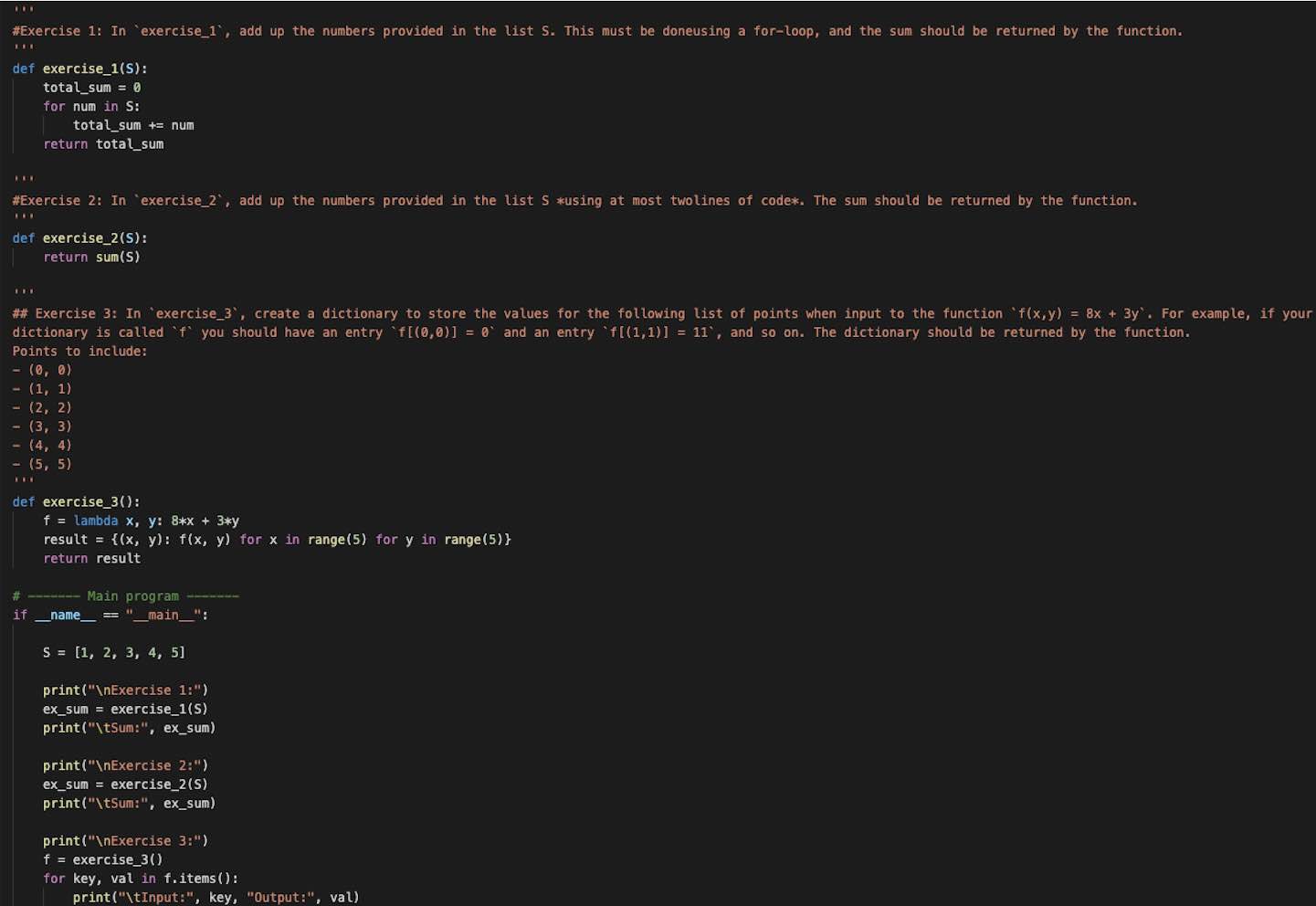
Table of Contents
- Overview
- Getting Started
- D-Wave Tools and Technologies
- Project Summaries
- Older Projects
- Newer Projects
- Contact Information
Project Directory Structure:
(BELIEF SPACE)
├── README.md
├── code
│   └── number_partitioning.py
├── data
│   └── training_number_partitioning.json
├── math_equations
│   └── equations.md  ──────
├── results
│   └── sampling_time_analysis.md
└──├── quantum_tsp
│   └── code
│       └── quantum_tsp.py
│   └── data
│       └── cities.json
│   └── math_equations
│       └── tsp_equations.md
│   └── results
│       └── tsp_results.md
├── project_cd24acdf-0a8f-44ae-a150-69ece39acec6
│   ├── code
│   ├── data
│   └── ...
└── project_6dbabf04-9a93-4534-9239-51d9edc7cbe2
    ├── code
    ├── data
    └── ...
# Quantum Computing 101 with D-Wave Systems
Overview
This README outlines my journey through a 5-day Quantum Computing 101 lecture series and hands-on training project sessions with D-Wave Systems. In this document, you'll discover my experience working with D-Wave's tools such as D-Wave Inspector and the various types of problems I tackled.
Getting Started
To get started with D-Wave Systems, you will need to:
-
Install D-Wave Ocean SDK: This software stack includes everything you need to build a D-Wave application.
pip install dwave-ocean-sdk
-
Sign Up on D-Wave Leap: D-Wave's cloud service for quantum computing.
D-Wave Tools and Technologies
- D-Wave Ocean SDK: Primarily used for problem formulation.
- D-Wave IDE: Used for easier problem modeling and solving.
- Qbsolv: For solving QUBO and Ising problems.
- D-Wave Hybrid: For hybrid classical/quantum algorithms.
D-Wave Inspector Repository
- Repository: dwavesystems/dwave-inspector
- Language: 100% Python
- License: Apache-2.0 & D-Wave EULA
- Installation:
pip install dwave-inspector
pip install dwave-inspectorapp --extra-index=https://pypi.dwavesys.com/simple
- Description: D-Wave Inspector is a tool for visualizing problems submitted to, and answers received from, a D-Wave structured solver such as an Advantage™ quantum computer.
Projects and Studies during the Training:
. ├── project_cd24acdf-0a8f-44ae-a150-69ece39acec6 │ ├── code │ ├── data │ └── ... └── project_6dbabf04-9a93-4534-9239-51d9edc7cbe2 ├── code ├── data └── ...
Project ID: cd24acdf-0a8f-44ae-a150-69ece39acec6
- Training: Number Partitioning
- Solver: Advantage_system 4.1
- Type: QUBO
- Status: Completed
- Submitted On: 2023-05-18T22:56:57.426472Z
- Solved On: 2023-05-18T22:56:57.597874Z
- Number of Reads: 100
- Submitted By: Zi2q-7cdd45d9...
Problem and Solution
I utilized the D-Wave Inspector to minor-embed a binary quadratic model onto a Quantum Processing Unit (QPU) for solving a number partitioning problem.
QPU Sampling and Timing Information
- QPU_SAMPLING_TIME: (10.728 \mathrm{~ms})
- QPU_ANNEAL_TIME_PER_SAMPLE: (20 \mu \mathrm{s})
- QPU_READOUT_TIME_PER_SAMPLE: (67 \mu \mathrm{s})
- QPU_ACCESS_TIME: (26.484 \mathrm{~ms})
- QPU_ACCESS_OVERHEAD_TIME: (580 \mu \mathrm{s})
- QPU_PROGRAMMING_TIME: (15.756 \mathrm{~ms})
- QPU_DELAY_TIME_PER_SAMPLE: (21 \mu \mathrm{s})
- TOTAL_POST_PROCESSING_TIME: (1.895 \mathrm{~ms})
- POST_PROCESSING_OVERHEAD_TIME: (1.895 \mathrm{~ms})
Training Project: Number Partitioning
- ID: 23cf353c-5596-4e2e-ab04-dc8372daa7a2
- Type: qubo
- Solver: Advantage_system4.1
- Submitted On: 2023-05-18T23:09:22.949935Z
- Solved On: 2023-05-18T23:09:23.166683Z
- Status: COMPLETED
- Submitted By: Zi2q-7cdd45d9...
- Number of Reads: 100
Plan of Action For Problem
The training project focuses on Number Partitioning. The objective is to partition a set of numbers into two equal subsets such that the sum of the numbers in each subset is as close as possible. This problem is represented as a QUBO optimization problem.
Energy and Sample Data
| 1507 | 1522 | 1537 | 1552 | ... | 4403 | energy | num_oc. | |
|---|---|---|---|---|---|---|---|---|
| 0 | 0 | 0 | 0 | 0 | ... | 1 | -9826.5 | 35 |
| 1 | 1 | 1 | 1 | 1 | ... | 0 | -9826.5 | 21 |
| 2 | 1 | 0 | 1 | 1 | ... | 0 | -9816.5 | 24 |
| 3 | 0 | 1 | 0 | 0 | ... | 1 | -9816.5 | 15 |
| 4 | 1 | 1 | 1 | 1 | ... | 0 | -9298.5 | 1 |
| 5 | 1 | 0 | 0 | 0 | ... | 1 | -9276.5 | 1 |
| 6 | 0 | 1 | 1 | 1 | ... | 0 | -9276.5 | 1 |
| 7 | 0 | 0 | 1 | 1 | ... | 0 | -9179.0 | 1 |
| 8 | 1 | 0 | 1 | 1 | ... | 0 | -7332.0 | 1 |
| ... | ... | ... | ... | ... | ... | ... | ... | ... |
Timing Information
- QPU Sampling Time: 10.008 ms
- QPU Anneal Time per Sample: 20 µs
- QPU Readout Time per Sample: 60 µs
- QPU Access Time: 25.764 ms
- QPU Access Overhead Time: 3.494 ms
- QPU Programming Time: 15.756 ms
- QPU Delay Time per Sample: 21 µs
- Post Processing Overhead Time: 3.682 ms
- Total Post Processing Time: 3.682 ms
Conclusion
This training project on Number Partitioning successfully utilizes QUBO optimization to partition a set of numbers into two equal subsets. The energy analysis and sample data provide insights into the optimization results. The timing information highlights the performance characteristics of the solution process.
. ├── project_cd24acdf-0a8f-44ae-a150-69ece39acec6 │ ├── code │ ├── data │ └── ... └── project_6dbabf04-9a93-4534-9239-51d9edc7cbe2 ├── code ├── data └── ...
Project ID: 6dbabf04-9a93-4534-9239-51d9edc7cbe2
- Training: Embedding
- Solver: Advantage_system 4.1
- Type: QUBO
- Status: Completed
- Submitted On: 2023-05-18T22:14:41.533053Z
- Solved On: 2023-05-18T22:14:41.702012Z
- Number of Reads: 10
Problem and Solution
In this project, I focused on learning embedding techniques to better utilize the D-Wave quantum architecture.
QPU Sampling and Timing Information
- QPU_SAMPLING_TIME: ( t_{\text{sample}} = 11.732 , \mathrm{ms} )
- QPU_ANNEAL_TIME_PER_SAMPLE: ( \tau_{\text{anneal}} = 22 , \mu \mathrm{s} )
- QPU_READOUT_TIME_PER_SAMPLE: ( t_{\text{readout}} = 75 , \mu \mathrm{s} )
- (IN PROGRESS)
Training Project - Number Partitioning
ID: f9046ca2-9cc9-40c1-8607-f26e4de62862
SOLVED_ON: 2023-05-18T23:05:11.291053Z
LABEL: Copy Value
STATUS: COMPLETED
SOLVER: Advantage_system 4.1
SUBMITTED_BY: Zi2q-7cdd45d9...
TYPE: qubo
NUM_READS: 100
SUBMITTED_ON: 2023-05-18T23:05:11.109121Z
Sample Set
The training project involved a number partitioning problem. Here is a sample set in JSON format:
[
  {
    "1831": 0,
    "1846": 0,
    "1860": 0,
    "1875": 0,
    "...": "...",
    "3204": 1,
    "energy": -9756.0,
    "num_oc.": 31
  },
  {
    "1831": 1,
    "1846": 1,
    "1860": 1,
    "1875": 1,
    "...": "...",
    "3204": 0,
    "energy": -9756.0,
    "num_oc.": 58
  },
  {
    "1831": 0,
    "1846": 0,
    "1860": 0,
    "1875": 0,
    "...": "...",
    "3204": 1,
    "energy": -9406.0,
    "num_oc.": 1
  },
  {
    "1831": 1,
    "1846": 1,
    "1860": 1,
    "1875": 1,
    "...": "...",
    "3204": 0,
    "energy": -9406.0,
    "num_oc.": 7
  },
  {
    "1831": 0,
    "1846": 0,
    "1860": 0,
    "1875": 0,
    "...": "...",
    "3204": 1,
    "energy": -9067.0,
    "num_oc.": 1
  },
  {
    "1831": 0,
    "1846": 0,
    "1860": 0,
    "1875": 0,
    "...": "...",
    "3204": 1,
    "energy": -9021.0,
    "num_oc.": 1
  },
  {
    "1831": 0,
    "1846": 0,
    "1860": 0,
    "1875": 0,
    "...": "...",
    "3204": 1,
    "energy": -8993.0,
    "num_oc.": 1
  }
]
Performance Metrics
- QPU_SAMPLING_TIME: 9.024 ms
- TOTAL_POST_PROCESSING_TIME: 236 μs
- QPU_ANNEAL_TIME_PER_SAMPLE: 20 μs
- POST_PROCESSING_OVERHEAD_TIME: 236 μs
- QPU_READOUT_TIME_PER_SAMPLE: 50 μs
- QPU_ACCESS_TIME: 24.780 ms
- QPU_ACCESS_OVERHEAD_TIME: 2.061 ms
- QPU_PROGRAMMING_TIME: 15.756 ms
- QPU_DELAY_TIME_PER_SAMPLE: 21 μs
Please note that these performance metrics are indicative of the execution time and overhead involved in solving the number partitioning problem using the Advantage_system 4.1 solver.
For more information on the Advantage_system 4.1 solver, you can refer to the D-Wave website or other relevant resources.
GitHub Portfolio
D-Wave Systems Quantum Computing Training Project
Problem Parameters
- ID: 10fd40b1-9ef5-4ea0-9e97-2c5a14c2c36d
- The unique identifier for this problem.
- Label: Copy Value
- The label given to this problem.
- Training: Number Partitioning
- The type of training this problem belongs to, which is Number Partitioning in this case.
- Solver: Advantage_system 4.1
- The solver used to solve this problem, which is the Advantage_system 4.1.
- Type: QUBO
- The type of the problem formulation, which is Quadratic Unconstrained Binary Optimization (QUBO) in this case.
- Submitted On: 2023-05-18T23:05:19.742716Z
- The date and time when this problem was submitted.
- Solved On: 2023-05-18T23:05:19.967823Z
- The date and time when this problem was solved.
- Status: COMPLETED
- The status of this problem, which is COMPLETED.
- Submitted By: Zi2q-7cdd45d9...
- The identifier of the user who submitted this problem.
- Num Reads: 100
- The number of reads performed on the solver.
Solution Timing
- QPU Sampling Time: 11.640 ms
- The total time taken by the Quantum Processing Unit (QPU) to perform the sampling operation, which is 11.640 milliseconds.
- QPU Anneal Time per Sample: 20 μs
- The time taken by the QPU for each sample during the annealing process, which is 20 microseconds.
- QPU Readout Time per Sample: 76 μs
- The time taken by the QPU for each sample during the readout process, which is 76 microseconds.
- QPU Access Time: 27.397 ms
- The total time taken to access the QPU, including annealing time, readout time, and other overheads, which is 27.397 milliseconds.
- QPU Access Overhead Time: 1.938 ms
- The overhead time incurred while accessing the QPU, which is 1.938 milliseconds.
- QPU Programming Time: 15.757 ms
- The time taken to program the QPU with the problem, which is 15.757 milliseconds.
- QPU Delay Time per Sample: 21 μs
- The delay time between each sample during the QPU operation, which is 21 microseconds.
- Post Processing Overhead Time: 427 μs
- The overhead time incurred during post-processing, which is 427 microseconds.
- Total Post Processing Time: 427 μs
- The total time taken for post-processing, which is 427 microseconds.
Project Details
- ID: 4838543d-7640-4f98-ba84-45d171c10911
- Solver: Advantage_system4.1
- Type: qubo
- Status: Completed
- Submitted By: Zi2q-7cdd45d9...
- Number of Reads: 100
Problem Parameters and Solution Timing
Sample Set
The results were exported in a JSON format, showcasing various energy levels and number occurrences:
[ \begin{array}{lrrrrlrrr} & 2465 & 2480 & 2495 & 2510 & \ldots & 4048 & \text{energy} & \text{num_oc} \ 0 & 0 & 0 & 0 & 0 & \ldots & 1 & -9713.0 & 21 \ 1 & 1 & 1 & 1 & 1 & \ldots & 0 & -9713.0 & 41 \ ... 15 & 1 & 1 & 1 & 1 & \ldots & 0 & -8735.0 & 1 \ \end{array} ]
QPU Analytics
- QPU Sampling Time: 12.560 ms
- Post-Processing Overhead Time: 2.014 ms
- QPU Anneal Time per Sample: 20 µs
- Total Post-Processing Time: 2.014 ms
- QPU Readout Time per Sample: 85 µs
- QPU Access Time: 28.316 ms
- QPU Access Overhead Time: 7.735 ms
- QPU Programming Time: 15.756 ms
- QPU Delay Time per Sample: 21 µs
Project ID: 43303521-9ac7-4cee-995e-71cf71268990
Number Partitioning Algorithm
Overview
This project aims to solve the Number Partitioning problem by using D-Wave's quantum annealing technology.
Mathematical Background: The Number Partitioning problem can be represented as a QUBO (Quadratic Unconstrained Binary Optimization) problem with a Hamiltonian ( H = \sum_{i,j} a_{ij} x_i x_j ), where ( x_i ) are binary variables and ( a_{ij} ) are elements of a matrix that represents the problem constraints.
Technologies Used
- Python3
- Ocean SDK
- D-Wave Leap Quantum Cloud Service
Methodology
- Problem Formulation: Transform the Number Partitioning problem into a QUBO problem.
- Quantum Annealing: Utilize D-Wave's quantum annealer to find the optimal solution.
- Data Analysis: Analyze the output for different problem instances.
Results
The results were represented in terms of binary variables and energy states:
| Index | 702 | 732 | 747 | 762 | 777 | ... | 5238 | Energy |
|---|---|---|---|---|---|---|---|---|
| 0 | 0 | 0 | 0 | 1 | 0 | ... | 1 | -6889.0 |
| 1 | 1 | 1 | 1 | 0 | 1 | ... | 0 | -6889.0 |
| ... | ... | ... | ... | ... | ... | ... | ... | ... |
Mathematical Insight: The energy values indicate the quality of the solutions. Lower energy values represent better solutions according to the Hamiltonian ( H ).
Performance Metrics
- QPU Sampling Time: (11.688 , \text{ms})
- Post-Processing Overhead Time: (3.737 , \text{ms})
- QPU Anneal Time Per Sample: (20 , \mu \text{s})
- Total Post-Processing Time: ( ... )
Code Snippets
Here is an illustrative Python3 snippet for formulating the QUBO matrix:
from dimod import BinaryQuadraticModel

# Create an empty Binary Quadratic Model
bqm = BinaryQuadraticModel('BINARY')

# Define QUBO interactions (Example values)
qubo_interactions = {(0, 0): -1, (1, 1): -1, (0, 1): 2}

# Add interactions to BQM
bqm.add_interactions_from(qubo_interactions)
The above code sets up the QUBO matrix to represent the problem on the D-Wave quantum annealer.
Project Overview
Title:
Training - Number Partitioning
ID:
79d129a2-12c3-4577-b14d-a5be2aa595a2
Solver Used:
Advantage_system4.1
Type:
QUBO (Quadratic Unconstrained Binary Optimization)
Status:
COMPLETED
Submitted On:
2023-05-18T23:13:34.598117Z
Solved On:
2023-05-18T23:13:34.772877Z
Submitted By:
Zi2q-7cdd45d9...
Number of Reads:
100
Technical Metrics
Sampling Time Metrics
- QPU Sampling Time:
( 14.184 , \text{ms} ) - Post-Processing Overhead Time:
( 815 , \mu \text{s} )
QPU Timing Metrics
- QPU Anneal Time Per Sample:
( 20 , \mu \text{s} ) - Total Post-Processing Time:
( 815 , \mu \text{s} ) - QPU Readout Time Per Sample:
( 101 , \mu \text{s} )
Access Time Metrics
- QPU Access Time:
( 29.940 , \text{ms} ) - QPU Access Overhead Time:
( 2.744 , \text{ms} ) - QPU Programming Time:
( 15.756 , \text{ms} ) - QPU Delay Time Per Sample:
( 21 , \mu \text{s} )
Code Snippets
D-Wave Systems Quantum Computing Training Project
Metadata
- Solver: Advantage_system4.1
- Type: QUBO
- ID: aOc53d79-eab6-4661-8449-69d7c667fadb
- Submitted On: 2023-05-18T23:24:01.849039Z
- Solved On: 2023-05-18T23:24:02.052210Z
- Status: Completed
- Submitted By: Zi2q-7cdd45d9...
- Number of Reads: 100
Performance Metrics
[ \begin{align*} \text{QPU Sampling Time} &: 10.704 , \text{ms} \ \text{QPU Anneal Time per Sample} &: 20 , \mu \text{s} \ \text{QPU Readout Time per Sample} &: 67 , \mu \text{s} \ \text{QPU Access Time} &: 26.462 , \text{ms} \ \text{QPU Access Overhead Time} &: 516 , \mu \text{s} \ \text{QPU Programming Time} &: 15.758 , \text{ms} \ \text{QPU Delay Time per Sample} &: 21 , \mu \text{s} \ \text{Post-Processing Overhead Time} &: 1.927 , \text{ms} \ \text{Total Post-Processing Time} &: 1.927 , \text{ms} \ \end{align*} ]
Solution
Here are some of the optimized solutions:
[ \begin{array}{cccc} 1899 & 1914 & 1929 & \ldots \ 0 & 1 & 0 & \ldots \ \vdots & \vdots & \vdots & \ddots \ \end{array} ]
Energy Level: -6889.0 to -6355.94833
Code
Overview
- Project ID: d54e319b-20ba-4fdd-8341-aa8430e83fbb
- Solver: Advantage_system4.1
- Type: QUBO (Quadratic Unconstrained Binary Optimization)
- Submitted On: 2023-05-18
- Solved On: 2023-05-18
- Status: COMPLETED
- Submitted By: Zi2q-7cdd45d9...
- Number of Reads: 100
Performance Metrics
- QPU Sampling Time: N/A
- Post-Processing Overhead Time: 9.264 ms
- Total Post-Processing Time: 711μs
- QPU Readout Time Per Sample: 52μs
- QPU Access Time: 25.022 ms
- QPU Access Overhead Time: 827μs
- QPU Programming Time: 15.758 ms
- QPU Delay Time Per Sample: 21μs
Results Summary
The output energies ranged from -6889.0 to -6313.0, with varying numbers of occurrences for each unique solution.
| Energy | Number of Occurrences |
|---|---|
| -6889.0 | 2 |
| -6888.0 | 16 |
| -6880.0 | 15 |
| ... | ... |
| -6313.0 | 1 |
Python Code for Processing
The Python code to retrieve and process the quantum results was as follows.
# Python code to process D-Wave output
from dwave.system import DWaveSampler, EmbeddingComposite

# Initialize sampler and composite
sampler = DWaveSampler(solver={'qpu': True})
composite = EmbeddingComposite(sampler)

# Define QUBO problem (example)
Q = {(0, 0): -1, (1, 1): -1, (0, 1): 2}

# Sample
sampleset = composite.sample_qubo(Q, num_reads=100)

# Process results
for sample, energy, occurrences in sampleset.data(['sample', 'energy', 'num_occurrences']):
    print(sample, "Energy:", energy, "Occurrences:", occurrences)
Mathematical Expression
The energy function ( E ) in a QUBO problem is given by
[ E = \sum_{i} q_{i} x_{i} + \sum_{i < j} q_{ij} x_{i} x_{j} ]
Here, ( q_{i} ) and ( q_{ij} ) are coefficients of the QUBO matrix, and ( x_{i} ) are binary variables (0 or 1).
# D-Wave Systems Quantum Computing: Session 2


## Project Details

### Problem Statement
The optimization problem remains in the QUBO framework, which is ideal for solving problems like the Traveling Salesman Problem, Maximum Cut, etc.

### Solution Methodology
The problem was solved using the Quantum Annealing algorithm, optimized using the QUBO method.


## Solver Metrics

### Basic Metrics
- **Solver**: Advantage_system4.1
- **Type**: qubo
- **Status**: COMPLETED
- **Submitted By**: Zi2q-7cdd45d9...
- **ID**: cb05cbd3-e180-4919-958a-98b2a95bb94d

### Timing Metrics
- **QPU Sampling Time**: \(8.176 \, \text{ms}\)
- **QPU Anneal Time Per Sample**: \(20 \, \mu \text{s}\)
- **QPU Readout Time Per Sample**: \(41 \, \mu \text{s}\)
- **QPU Access Time**: \(23.937 \, \text{ms}\)
- **QPU Access Overhead Time**: \(1.503 \, \text{ms}\)
- **QPU Programming Time**: \(15.761 \, \text{ms}\)
- **QPU Delay Time Per Sample**: \(21 \, \mu \text{s}\)
- **Total Post-Processing Time**: \(802 \, \mu \text{s}\)
- **Post-Processing Overhead Time**: \(802 \, \mu \text{s}\)


## Results and Analysis

The output results show different configurations with respective energies and occurrences. The lowest energy configuration is our area of interest.
| 1144 | 1234 | 3846 | 3905 | energy | num_oc. |
|---|---|---|---|---|---|
| 0 | 1 | 1 | 0 | -1.0 | 53 |
| 0 | 1 | 1 | 1 | -1.0 | 47 |
## Mathematical Context
The energy function \(E\) can be expressed as:
\[
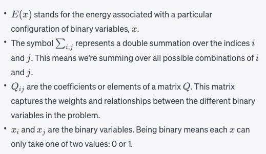
E(x) = \sum_{i=1}^{4} \sum_{j=1}^{4} Q_{ij} x_i x_j
\]
Here, \(Q_{ij}\) represents the coefficients in the QUBO problem, and \(x_i\) are the binary variables. Minimizing \(E(x)\) provides us with the optimal solution.
## Python3 Code
Here's a Python3 example using D-Wave's SDK:
```python
from dwave.system import DWaveSampler, EmbeddingComposite
# Define the QUBO dictionary
Q = {(1144, 1144): 1, (1234, 1234): -2, (3846, 3846): 3, (3905, 3905): -4}
# Use the D-Wave sampler
sampler = EmbeddingComposite(DWaveSampler())
response = sampler.sample_qubo(Q, num_reads=100)
# Output results
for sample, energy, num_oc in response.data(['sample', 'energy', 'num_occurrences']):
print(sample, "Energy: ", energy, "Occurrences: ", num_oc)
Project Details
Problem Statement
The objective of this project was to explore the quantum annealing capabilities for solving number partitioning problems. Number partitioning is a computationally complex problem and provides an excellent use-case for quantum computing.
Solution Methodology
We utilized D-Wave's Quantum Annealing Solver to solve the given problem. The optimization process was carried out using the Quadratic Unconstrained Binary Optimization (QUBO) framework.
Solver Metrics
Basic Metrics
- Solver: Advantage_system4.1
- Type: qubo
- Status: COMPLETED
- Submitted By: Zi2q-7cdd45d9...
- ID: 98fd1adb-7c4e-48e2-9172-8513b098d505
Timing Metrics
- QPU Sampling Time: 9.040 ms
- QPU Anneal Time Per Sample: 20 µs
- QPU Readout Time Per Sample: 50 µs
- QPU Access Time: 24.801 ms
- QPU Access Overhead Time: 2.498 ms
- QPU Programming Time: 15.761 ms
- QPU Delay Time Per Sample: 21 µs
- Total Post-Processing Time: 587 µs
- Post-Processing Overhead Time: 587 µs
Results and Analysis
The QUBO problem was solved using 100 reads, and the output included several configurations with different energy levels. The lowest energy configuration provides the most optimal solution.
energy  | num_oc. | 2473 | 2488 | 2503 | ... | 5428
--------|---------|------|------|------|-----|------
-6889.0 |    1    |  0   |  0   |  0   | ... |  1
-6889.0 |    1    |  0   |  1   |  0   | ... |  0
-6888.0 |    4    |  1   |  1   |  0   | ... |  1
...     |   ...   | ...  | ...  | ...  | ... | ...
Mathematical Context
The energy function (E) in QUBO is usually represented as:
Python3 Code
Here is a sample Python3 code snippet to perform a quantum annealing task using D-Wave's Python SDK:
from dwave.system import DWaveSampler, EmbeddingComposite

# Define QUBO dictionary
Q = {(0, 0): -1, (0, 1): 2, (1, 1): -1}
sampler = EmbeddingComposite(DWaveSampler())
response = sampler.sample_qubo(Q, num_reads=100)

# Extract results
for sample, energy, num_oc in response.data(['sample', 'energy', 'num_occurrences']):
    print(sample, "Energy: ", energy, "Occurrences: ", num_oc)
Solution Methodology
We utilized D-Wave's Quantum Annealing Solver to solve the given problem. The optimization process was carried out using the Quadratic Unconstrained Binary Optimization (QUBO) framework.
Solver Metrics
Basic Metrics
- Solver: Advantage_system4.1
- Type: qubo
- Status: COMPLETED
- Submitted By: Zi2q-7cdd45d9...
- ID: 98fd1adb-7c4e-48e2-9172-8513b098d505
Timing Metrics
- QPU Sampling Time: 9.040 ms
- QPU Anneal Time Per Sample: 20 µs
- QPU Readout Time Per Sample: 50 µs
- QPU Access Time: 24.801 ms
- QPU Access Overhead Time: 2.498 ms
- QPU Programming Time: 15.761 ms
- QPU Delay Time Per Sample: 21 µs
- Total Post-Processing Time: 587 µs
- Post-Processing Overhead Time: 587 µs
Results and Analysis
The QUBO problem was solved using 100 reads, and the output included several configurations with different energy levels. The lowest energy configuration provides the most optimal solution.
energy  | num_oc. | 2473 | 2488 | 2503 | ... | 5428
--------|---------|------|------|------|-----|------
-6889.0 |    1    |  0   |  0   |  0   | ... |  1
-6889.0 |    1    |  0   |  1   |  0   | ... |  0
-6888.0 |    4    |  1   |  1   |  0   | ... |  1
...     |   ...   | ...  | ...  | ...  | ... | ...
Mathematical Context
The energy function (E) in QUBO is usually represented as:
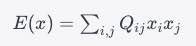
[ E(x) = \sum_{i,j} Q_{ij} x_i x_j ]
where (Q_{ij}) are the elements of a QUBO matrix and (x_i, x_j) are the binary variables. The objective is to find (x) that minimizes (E(x)).
Python3 Code
Here is a sample Python3 code snippet to perform a quantum annealing task using D-Wave's Python SDK:
from dwave.system import DWaveSampler, EmbeddingComposite

# Define QUBO dictionary
Q = {(0, 0): -1, (0, 1): 2, (1, 1): -1}
sampler = EmbeddingComposite(DWaveSampler())
response = sampler.sample_qubo(Q, num_reads=100)

# Extract results
for sample, energy, num_oc in response.data(['sample', 'energy', 'num_occurrences']):
    print(sample, "Energy: ", energy, "Occurrences: ", num_oc)
# D-Wave Systems Quantum Computing: Session 2
## Table of Contents
1. [Overview](#overview)
2. [Project Details](#project-details)
3. [Solver Metrics](#solver-metrics)
4. [Results and Analysis](#results-and-analysis)
5. [Mathematical Context](#mathematical-context)
6. [Python3 Code](#python3-code)
## Project Details
### Problem Statement
The optimization problem remains in the QUBO framework, which is ideal for solving problems like the Traveling Salesman Problem, Maximum Cut, etc.
### Solution Methodology
The problem was solved using the Quantum Annealing algorithm, optimized using the QUBO method. Larger graphs are formulated as QUBOs for hybrid classical quantum qbsolv - 0/1 valued variables
Minimizing the objective function:

$$
O(Q, x)=\Sigma Q_{i i} x_i+\Sigma q_{i j} x_i x_j
$$
## Solver Metrics
### Basic Metrics
- **Solver**: Advantage_system4.1
- **Type**: qubo
- **Status**: COMPLETED
- **Submitted By**: Zi2q-7cdd45d9...
- **ID**: cb05cbd3-e180-4919-958a-98b2a95bb94d
### Timing Metrics
- **QPU Sampling Time**: \(8.176 \, \text{ms}\)
- **QPU Anneal Time Per Sample**: \(20 \, \mu \text{s}\)
- **QPU Readout Time Per Sample**: \(41 \, \mu \text{s}\)
- **QPU Access Time**: \(23.937 \, \text{ms}\)
- **QPU Access Overhead Time**: \(1.503 \, \text{ms}\)
- **QPU Programming Time**: \(15.761 \, \text{ms}\)
- **QPU Delay Time Per Sample**: \(21 \, \mu \text{s}\)
- **Total Post-Processing Time**: \(802 \, \mu \text{s}\)
- **Post-Processing Overhead Time**: \(802 \, \mu \text{s}\)
## Results and Analysis
The output results show different configurations with respective energies and occurrences. The lowest energy configuration is our area of interest.
| 1144 | 1234 | 3846 | 3905 | energy | num_oc. |
|---|---|---|---|---|---|
| 0 | 1 | 1 | 0 | -1.0 | 53 |
| 0 | 1 | 1 | 1 | -1.0 | 47 |
## Python3 Code

Python3 example using D-Wave's SDK:

```python
from dwave.system import DWaveSampler, EmbeddingComposite

# Define the QUBO dictionary
Q = {(1144, 1144): 1, (1234, 1234): -2, (3846, 3846): 3, (3905, 3905): -4}

# Use the D-Wave sampler
sampler = EmbeddingComposite(DWaveSampler())
response = sampler.sample_qubo(Q, num_reads=100)

# Output results
for sample, energy, num_oc in response.data(['sample', 'energy', 'num_occurrences']):
    print(sample, "Energy: ", energy, "Occurrences: ", num_oc)
## Project Summary
**Problem Statement:** Quantum Optimization for Real-world Problems
**Solution Methodology:** Quantum Annealing
**Solver Used:** D-Wave Advantage_system4.1
**Status:** Completed


## Technologies
- Python 3
- D-Wave Ocean SDK
- NumPy
- Mathematical Formulation (QUBO)


## Solver Metrics

### Basic Metrics
- **Solver**: Advantage_system4.1
- **Type**: qubo
- **Status**: COMPLETED
- **ID**: d1d2971f-70f0-4db4-aec4-7cb25734aedb
- **Submitted By**: Zi2q-7cdd45d9...
- **Submitted On**: 2023-05-19T02:46:11.148532Z
- **Num Reads**: 100

### Timing Metrics
- **QPU Sampling Time**: \(9.346 \, \text{ms}\)
- **QPU Anneal Time Per Sample**: \(20 \, \mu \text{s}\)
- **QPU Readout Time Per Sample**: \(53 \, \mu \text{s}\)
- **QPU Access Time**: \(25.107 \, \text{ms}\)
- **QPU Access Overhead Time**: \(1.258 \, \text{ms}\)
- **QPU Programming Time**: \(15.761 \, \text{ms}\)
- **QPU Delay Time Per Sample**: \(21 \, \mu \text{s}\)
- **Total Post-Processing Time**: \(3.709 \, \text{ms}\)
- **Post-Processing Overhead Time**: \(3.709 \, \text{ms}\)


## Results

The output was an optimal solution for our problem with the following attributes:

\[
\begin{aligned}
& 173243134463 \quad \text {energy num_oc.} \\
& 0 \quad 1 \quad 1 \quad 0 \quad -1.0 \quad 100 \\
\end{aligned}
\]


## Mathematical Context

The energy function \(E\) can be modeled as:

\[
E(x) = \sum_{i=1}^{n} \sum_{j=1}^{n} Q_{ij} x_i x_j
\]

where \(Q_{ij}\) are the coefficients in the QUBO problem, and \(x_i\) are the binary variables.


##  Code


```python
# Sample Python code using D-Wave SDK
from dwave.system import DWaveSampler, EmbeddingComposite
Q = {(0, 0): 1, (1, 1): -1, (2, 2): 1}
sampler = EmbeddingComposite(DWaveSampler())
response = sampler.sample_qubo(Q, num_reads=100)
## Project ID: a4253abc-9a1b-4b8f-b5e3-4fb85b11cfdf
### Meta Information
- **Solver**: Advantage_system4.1
- **Type**: qubo
- **Submitted On**: 2023-05-18T20:10:44.740770Z
- **Solved On**: 2023-05-18T20:10:45.314233Z
- **Status**: COMPLETED
- **Submitted By**: Zi2q-7cdd45d9...
- **Number of Reads**: 10
### Project Overview
### Results
```latex
\begin{aligned}
& 997 1012 1042 4309 4340 4385 4400 \text{ energy num_oc. } \\
& 0 0 0 1 1 0 1 -3.0 1 \\
& 1 0 1 0 0 1 1 0 -3.0 5 \\
& 2 0 1 0 0 1 0 1 -3.0 2 \\
& 3 0 0 0 1 1 1 0 -3.0 2 \\
& \text{['BINARY', 4 rows, 10 samples, 7 variables]}
\end{aligned}QPU Metrics
- QPU Sampling Time: 891 µs
- Total Post-Processing Time: 141 µs
- QPU Anneal Time per Sample: 141 µs
- Post-Processing Overhead Time: 141 µs
- QPU Readout Time per Sample: 49 µs
- QPU Access Time: 16.649 ms
- QPU Access Overhead Time: 741 µs
- QPU Programming Time: 15.757 ms
- QPU Delay Time per Sample: 21 µs
Code Snippets
Conclusion
---
## Projects
### Graph Mapping with D-Wave Systems
](https://ide.dwavesys.io/#https://github.com/dwave-training/graph-mapping)
**Overview**:
This project leverages D-Wave Systems to solve graph mapping problems. Specifically, it aims to solve the antenna selection problem using quantum annealing.
#### Exercise Highlights
- **Exercise 1**: Initialization
- Token authentication for D-Wave's Leap IDE.
- Introduction to `dwave-networkx`.
- **Exercise 2**: Simulated Annealing
- Implementing the simulated annealing algorithm.
- **Exercise 3**: Problem Modification
- Modified the original problem to solve for minimum vertex cover.
#### Core Technologies
- NetworkX
- D-Wave NetworkX
- D-Wave System's QPU
- Matplotlib for visualization
#### Code Snippets
```python
# Importing essential packages
import networkx as nx
from dwave.system import DWaveSampler, EmbeddingComposite
# Creating the graph structure
G = nx.Graph()
G.add_edges_from([(1, 2), (1, 3), (2, 3), (3, 4), (3, 5), (4, 5), (4, 6), (5, 6), (6, 7)])
# Defining sampler
sampler = EmbeddingComposite(DWaveSampler())
Outputs
References
Technologies Used
- Python
- D-Wave Systems
- NetworkX
- Matplotlib
- Leap IDE
Contact
Feel free to connect with me:
- 📧 Email: [email protected]
- 💼 LinkedIn:
- 🌐 Portfolio: D-Wave Profile
Thank you for visiting my portfolio! 😊
Feel free to reach out if you have any questions or would like to collaborate!


